library(ggplot2)

te_pal <- list(forest = "#275139", green = "#2f8f63", sage = "#93a87f",
               clay = "#b5534e", gold = "#cda23f", line = "#dad9ca",
               ink = "#16241d", paper = "#f5f4ee")

theme_te <- function() {
  theme_minimal(base_size = 12) +
    theme(panel.grid.minor = element_blank(),
          panel.grid.major = element_line(colour = "#e7e6dc"),
          plot.background = element_rect(fill = "#f5f4ee", colour = NA),
          panel.background = element_rect(fill = "#f5f4ee", colour = NA),
          plot.title = element_text(face = "bold", colour = te_pal$ink),
          axis.title = element_text(colour = "#2c3a31"))
}Multiple matrix regression with MMRR
R
landscape genetics
hypothesis testing
ecology tutorial
ggplot2
Regress a genetic distance matrix on several landscape distances in base R, permute rows and columns together, and measure the type I error each test has.
The previous tutorial built a pairwise genetic distance and three competing landscape distances, and stopped there on purpose: no p-value. This one supplies the missing half. The response is a matrix, the predictors are matrices, and the temptation is to stack their lower triangles into columns and call lm().
That works for the coefficients and fails for everything else. Fifteen sites give 105 pairs but only 15 independent things were sampled, and every site appears in 14 of those pairs. Multiple matrix regression with randomisation (MMRR) keeps the least-squares fit and replaces the p-value with a permutation that respects the sharing. This tutorial writes it in base R and then measures how often each candidate test rejects a predictor that has no effect.
The dependence, concretely
Write the genetic distance between sites i and j as a site term plus a pair term. If site i happens to be genetically unusual, every one of its 14 pairs is shifted in the same direction, so the residuals of the vectorised regression come in correlated blocks. Ordinary standard errors assume 105 independent draws, count that shared shift as information, and come out too small.
MMRR’s answer is to permute the site labels. Draw one random ordering of the sites and apply it to the rows and the columns of the response matrix at once. The result is still a valid distance matrix with the same site structure, but the alignment between the response and the predictors is destroyed. Repeat, and the spread of the permuted coefficients is the null the test needs.
A generator with a known answer
To check a test you need data whose truth you set. This generator is deliberately not a population-genetic simulation: it places k sites at random in a unit square, builds geographic distance and one second predictor, and writes the genetic distance directly as an intercept plus standardised predictors plus noise. The point is that the coefficients are known, so a rejection rate can be compared with the rate the test advertises.
The noise is the part that matters. It has a site component drawn once per site and added to all of that site’s pairs, plus a pair component. Without the site component the vectorised pairs really would be independent and lm() would be correct; with it, they are not, which is the situation any real distance matrix is in.
zs <- function(v) (v - mean(v)) / sd(v)

lower_of <- function(m) m[lower.tri(m)]

sym_fill <- function(v, k) {
  out <- matrix(0, k, k)
  out[lower.tri(out)] <- v
  out + t(out)
}

site_field <- function(coords, range_par) {
  k <- nrow(coords)
  d_xy <- as.matrix(dist(coords))
  as.vector(t(chol(exp(-(d_xy / range_par)^2) + diag(1e-6, k))) %*% rnorm(k))
}

gen_pairs <- function(k = 15, b0 = 3.5, b1 = 0.6, b2 = 0,
                      sd_site = 0.6, sd_pair = 0.25,
                      second = "field", range_par = 0.6) {
  coords <- cbind(runif(k), runif(k))
  d_geo <- as.matrix(dist(coords))
  x2 <- if (second == "barrier") {
    side <- as.numeric(coords[, 1] > 0.5)
    abs(outer(side, side, "-"))
  } else {
    z <- site_field(coords, range_par)
    abs(outer(z, z, "-"))
  }
  site_eff <- rnorm(k, 0, sd_site)
  n_pair <- k * (k - 1) / 2
  y_low <- b0 + b1 * zs(lower_of(d_geo)) + b2 * zs(lower_of(x2)) +
    lower_of(outer(site_eff, site_eff, "+")) + rnorm(n_pair, 0, sd_pair)
  list(y = sym_fill(y_low, k), geo = d_geo, x2 = x2)
}

n_site <- 15
cat("sites in the default design:", n_site,
    " pairs:", n_site * (n_site - 1) / 2,
    " pairs sharing any one site:", n_site - 1, "\n")
sites in the default design: 15 pairs: 105 pairs sharing any one site: 14 cat("residual degrees of freedom, two predictors and an intercept:",
n_site * (n_site - 1) / 2 - 3, "\n")residual degrees of freedom, two predictors and an intercept: 102 The second predictor comes in two flavours. A barrier splits the square in half, which is the familiar river or road; a smooth Gaussian random field over the same coordinates gives a spatially structured nuisance variable, correlated with geographic distance by construction rather than by biology. The type I error study needs the second kind.
MMRR by hand
Two pieces. perm_index turns a batch of site orderings into linear indices into the response matrix, so that one random ordering permutes rows and columns together in a single gather. mmrr fits by least squares and reuses the precomputed cross product for every permutation, since only the response is reshuffled.
perm_index <- function(k, n_perm) {
  low <- which(lower.tri(matrix(0, k, k)), arr.ind = TRUE)
  p_mat <- vapply(seq_len(n_perm), function(b) sample.int(k), integer(k))
  (p_mat[low[, 2], ] - 1) * k + p_mat[low[, 1], ]
}

mmrr <- function(y_mat, x_mats, n_perm = 999, idx = NULL) {
  k <- nrow(y_mat)
  n_pair <- k * (k - 1) / 2
  x_des <- cbind(1, vapply(x_mats, function(m) zs(lower_of(m)),
                           numeric(n_pair)))
  xtx_inv <- solve(crossprod(x_des))
  proj <- xtx_inv %*% t(x_des)
  n_par <- ncol(x_des)
  stats_of <- function(y_cols) {
    beta <- proj %*% y_cols
    rss <- colSums((y_cols - x_des %*% beta)^2)
    list(beta = beta,
         r2 = 1 - rss / colSums(sweep(y_cols, 2, colMeans(y_cols))^2),
         tstat = beta / sqrt(outer(diag(xtx_inv), rss / (n_pair - n_par))))
  }
  obs <- stats_of(cbind(lower_of(y_mat)))
  if (is.null(idx)) idx <- perm_index(k, n_perm)
  nul <- stats_of(matrix(y_mat[idx], n_pair, ncol(idx)))
  list(beta = as.vector(obs$beta), tstat = as.vector(obs$tstat),
       r2 = obs$r2, null_beta = nul$beta,
       p_perm = (1 + rowSums(abs(nul$tstat) >=
                               abs(as.vector(obs$tstat)))) / (ncol(idx) + 1),
       p_lm = 2 * pt(-abs(as.vector(obs$tstat)), n_pair - n_par),
       p_r2 = (1 + sum(nul$r2 >= obs$r2)) / (ncol(idx) + 1))
}
The intercept is not testable this way. Permuting rows and columns together reorders the pairs without changing the values in the lower triangle, so the response mean, and with standardised predictors the intercept itself, is the same in every permutation. The permutation p printed for the intercept row below is an artefact of that: it comes from the t statistic, whose denominator uses a residual variance that does change under permutation, not from the coefficient, which is constant.
Fit one dataset of 18 sites where geographic distance has a coefficient of 0.55 and a barrier has 0.3.
n_demo <- 18
n_perm_demo <- 999
cat("demonstration dataset:", n_demo, "sites,",
    n_demo * (n_demo - 1) / 2, "pairs,", n_perm_demo, "permutations\n")
demonstration dataset: 18 sites, 153 pairs, 999 permutationsset.seed(95)
demo <- gen_pairs(k = n_demo, b0 = 3.5, b1 = 0.55, b2 = 0.30,
sd_site = 0.6, sd_pair = 0.25, second = "barrier")
fit <- mmrr(demo$y, list(geography = demo$geo, barrier = demo$x2),
n_perm = n_perm_demo)
print(data.frame(term = c("intercept", "geography", "barrier"),
truth = c(3.5, 0.55, 0.3),
estimate = round(fit$beta, 4),
t_value = round(fit$tstat, 3),
p_permutation = round(fit$p_perm, 4),
p_ordinary_lm = signif(fit$p_lm, 3)), row.names = FALSE) term truth estimate t_value p_permutation p_ordinary_lm
intercept 3.50 3.4579 46.895 0.001 1.64e-91
geography 0.55 0.5623 5.789 0.001 4.01e-08
barrier 0.30 0.2865 2.949 0.036 3.70e-03cat("r squared:", round(fit$r2, 4), " permutation p for r squared:",
round(fit$p_r2, 4), "\n")r squared: 0.4251 permutation p for r squared: 0.001 cat("correlation between the two predictor vectors:",
round(cor(lower_of(demo$geo), lower_of(demo$x2)), 4), "\n")correlation between the two predictor vectors: 0.6481 cat("barrier, ordinary lm p:", round(fit$p_lm[3], 4),
" permutation p:", round(fit$p_perm[3], 4), "\n")barrier, ordinary lm p: 0.0037 permutation p: 0.036 The coefficients come out at 0.5623 against a true 0.55 for geography and 0.2865 against a true 0.3 for the barrier. The r squared of 0.4251 has a permutation p of 0.001, the smallest value 999 permutations can produce.
Here the barrier is where the two p-values part company. Ordinary least squares gives 0.0037 and the permutation gives 0.036, much weaker for the same coefficient and the same t of 2.949. Nothing about the fit changed; only the reference distribution did.
null_df <- rbind(
  data.frame(value = fit$null_beta[2, ], term = "geographic distance"),
  data.frame(value = fit$null_beta[3, ], term = "barrier"))
obs_df <- data.frame(term = c("geographic distance", "barrier"),
                     value = fit$beta[2:3])
null_df$term <- factor(null_df$term, levels = obs_df$term)
obs_df$term <- factor(obs_df$term, levels = obs_df$term)

ggplot(null_df, aes(value)) +
  geom_histogram(bins = 40, fill = te_pal$sage, colour = "white",
                 linewidth = 0.2) +
  geom_vline(data = obs_df, aes(xintercept = value), colour = te_pal$clay,
             linewidth = 1) +
  facet_wrap(~term) +
  labs(title = "What the coefficients look like with the labels shuffled",
       subtitle = "999 permutations of the site order, applied to rows and columns together",
       x = "coefficient under permutation", y = "permutations") +
  theme_te()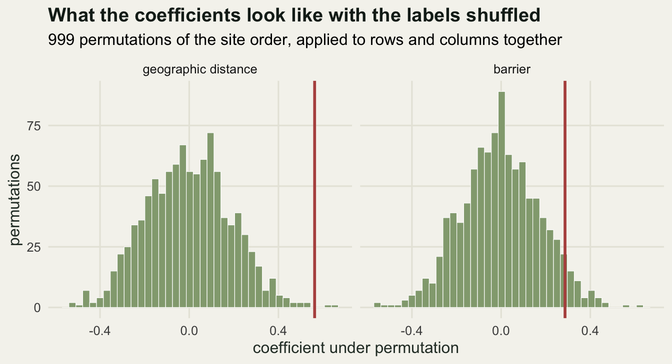
Three ways to get a p-value from one fit
A simple Mantel test is the third option, and the previous tutorial in this cluster covers how it works. Run it against each predictor separately and compare all three.
mantel_simple <- function(y_mat, x_mat, n_perm = 999) {
  k <- nrow(y_mat)
  n_pair <- k * (k - 1) / 2
  xv <- zs(lower_of(x_mat))
  obs <- sum(zs(lower_of(y_mat)) * xv) / (n_pair - 1)
  y_perm <- matrix(y_mat[perm_index(k, n_perm)], n_pair, n_perm)
  nul <- as.vector(crossprod(xv, apply(y_perm, 2, zs))) / (n_pair - 1)
  c(r = obs, p = (1 + sum(abs(nul) >= abs(obs))) / (n_perm + 1))
}

man_geo <- mantel_simple(demo$y, demo$geo)
man_bar <- mantel_simple(demo$y, demo$x2)
print(data.frame(
  predictor = c("geography", "barrier"),
  mantel_r = round(c(man_geo[1], man_bar[1]), 4),
  mantel_p = round(c(man_geo[2], man_bar[2]), 4),
  mmrr_coefficient = round(fit$beta[2:3], 4),
  mmrr_p = round(fit$p_perm[2:3], 4),
  lm_p = signif(fit$p_lm[2:3], 3)), row.names = FALSE)
predictor mantel_r mantel_p mmrr_coefficient mmrr_p lm_p
geography 0.6260 0.001 0.5623 0.001 4.01e-08
barrier 0.5447 0.001 0.2865 0.036 3.70e-03The simple Mantel correlations are 0.6260 for geography and 0.5447 for the barrier, both with p = 0.001. Taken at face value that is two significant landscape effects, but the two predictors correlate at 0.6481 with each other, so a marginal test cannot say whether the barrier does anything that distance does not already do. That is the question MMRR answers, and its answer for the barrier is 0.036.
So the same barrier, in this one dataset, supports a p of 0.001, 0.0037 or 0.036 depending on which test is run. Which of them is right is not a matter of taste, because a test makes a checkable promise: reject a true null five per cent of the time.
How often does each test cry wolf?
Now generate data where genetic distance depends on geography alone. The second predictor is the smooth field: spatially structured, correlated with geographic distance, and with a coefficient of exactly zero. Any rejection is a false one.
The partial Mantel test goes in here as implemented in the literature: residualise both the response and the tested predictor on the other predictor, correlate the residuals, and permute the rows and columns of the response.
partial_mantel <- function(y_mat, x_mat, z_mat, idx) {
  k <- nrow(y_mat)
  n_pair <- k * (k - 1) / 2
  z_des <- cbind(1, zs(lower_of(z_mat)))
  res_of <- function(mm) mm - z_des %*% qr.solve(z_des, mm)
  rx <- res_of(cbind(zs(lower_of(x_mat))))
  ry <- res_of(cbind(lower_of(y_mat),
                     matrix(y_mat[idx], n_pair, ncol(idx))))
  cc <- as.vector(crossprod(rx, ry)) / sqrt(sum(rx^2) * colSums(ry^2))
  c(r = cc[1], p = (1 + sum(abs(cc[-1]) >= abs(cc[1]))) / (ncol(idx) + 1))
}

run_study <- function(n_rep, b1, b2, k_site = n_site, n_perm = 499) {
  out <- matrix(NA_real_, n_rep, 5)
  for (rr in seq_len(n_rep)) {
    dat <- gen_pairs(k = k_site, b1 = b1, b2 = b2, second = "field")
    idx <- perm_index(k_site, n_perm)
    ff <- mmrr(dat$y, list(geo = dat$geo, nuis = dat$x2), idx = idx)
    pm <- partial_mantel(dat$y, dat$x2, dat$geo, idx)
    out[rr, ] <- c(ff$p_lm[3], pm[2], ff$p_perm[3], ff$tstat[3],
                   cor(lower_of(dat$geo), lower_of(dat$x2)))
  }
  out
}

n_rep_main <- 400
cat("replicates:", n_rep_main, " sites per replicate:", n_site,
    " permutations per replicate:", 499, "\n")
replicates: 400 sites per replicate: 15 permutations per replicate: 499 set.seed(3141)
study <- run_study(n_rep = n_rep_main, b1 = 0.6, b2 = 0)
rates <- colMeans(study[, 1:3] < 0.05)
type_one <- data.frame(
method = c("ordinary lm", "partial Mantel", "MMRR"),
rejection_rate = round(rates, 4),
mc_standard_error = round(sqrt(rates * (1 - rates) / n_rep_main), 4))
print(type_one, row.names = FALSE) method rejection_rate mc_standard_error
ordinary lm 0.2675 0.0221
partial Mantel 0.0900 0.0143
MMRR 0.0900 0.0143cat("the same rejection rates as percentages:",
paste(round(100 * rates, 2), collapse = ", "), "\n")the same rejection rates as percentages: 26.75, 9, 9 cat("mean correlation of nuisance with geographic distance:",
round(mean(study[, 5]), 4), "\n")mean correlation of nuisance with geographic distance: 0.4148 cat("largest difference between the partial Mantel and MMRR p values:",
max(abs(study[, 2] - study[, 3])), "\n")largest difference between the partial Mantel and MMRR p values: 0 cat("ordinary lm rate divided by the nominal 0.05:",
round(rates[1] / 0.05, 2), "\n")ordinary lm rate divided by the nominal 0.05: 5.35 cat("standard deviation of the ordinary t statistic:",
round(sd(study[, 4]), 4), " assumed:",
round(sqrt(102 / 100), 4), "\n")standard deviation of the ordinary t statistic: 1.8331 assumed: 1.01 Three rejection rates against a nominal 0.05, and none of them is 0.05. Ordinary least squares rejects a null predictor 26.75 per cent of the time, 5.35 times the nominal rate, with a Monte Carlo standard error of 0.0221. The permutation tests reject 9 per cent of the time, standard error 0.0143. The nuisance predictor correlates with geographic distance at 0.4148 on average, which is an ordinary amount of spatial structure for an environmental variable.
The partial Mantel and MMRR rows are not similar, they are identical: the largest difference between the two p-values over 400 replicates is 0. That is algebra, not luck. The partial correlation between the response and one predictor, holding the others fixed, is a monotone function of that predictor’s t statistic in the multiple regression, so with the same permutations the two tests order the null the same way and return the same p-value. When a partial Mantel controls for everything else in the model, it is MMRR’s coefficient test under a different name. MMRR earns its place by scaling past two predictors and by reporting coefficients you can compare, not by having a better null.
type_one$method <- factor(type_one$method, levels = type_one$method)

ggplot(type_one, aes(method, rejection_rate)) +
  geom_hline(yintercept = 0.05, linetype = "dashed", colour = "grey40") +
  geom_errorbar(aes(ymin = rejection_rate - 2 * mc_standard_error,
                    ymax = rejection_rate + 2 * mc_standard_error),
                width = 0.12, colour = te_pal$forest) +
  geom_point(colour = te_pal$forest, size = 3.4) +
  coord_cartesian(ylim = c(0, 0.32)) +
  labs(title = "Only the permutation comes near the promised five per cent",
       subtitle = "spatially structured predictor with a true coefficient of zero, 400 replicates",
       x = NULL, y = "rejection rate at alpha 0.05") +
  theme_te()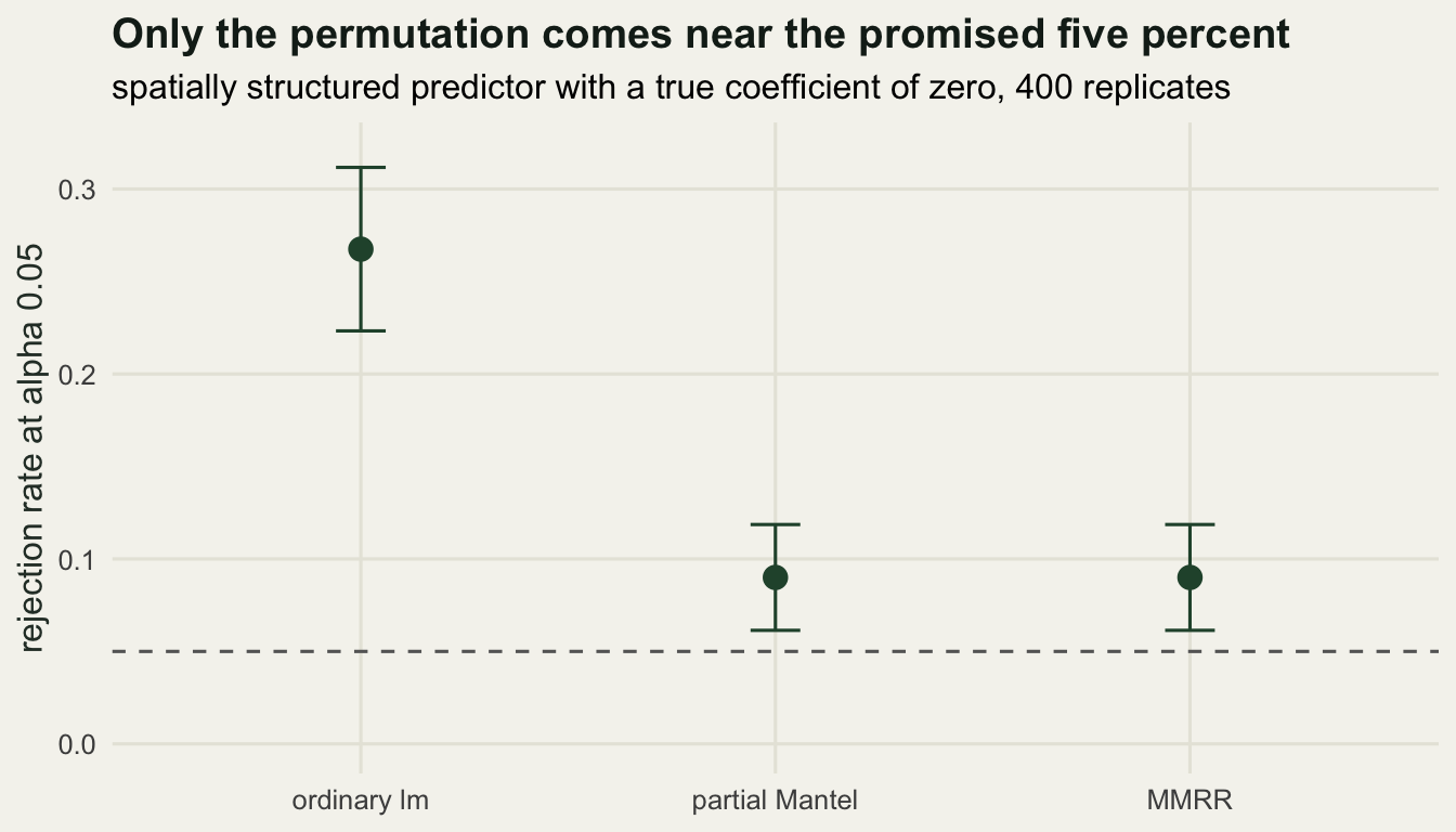
Why the ordinary test fails, in one picture
The mechanism is visible in the t statistic itself. The ordinary test compares it with a t distribution on 102 degrees of freedom, whose standard deviation is 1.01. The actual sampling distribution has a standard deviation of 1.8331, so the reference curve is far too narrow and the tails are where the false positives come from.
t_df <- data.frame(t_value = study[, 4])
crit <- qt(0.975, 102)
curve_df <- data.frame(t_value = seq(-6, 6, length.out = 400))
curve_df$density <- dt(curve_df$t_value, 102)

ggplot(t_df, aes(t_value)) +
  geom_histogram(aes(y = after_stat(density)), bins = 40,
                 fill = te_pal$sage, colour = "white", linewidth = 0.2) +
  geom_line(data = curve_df, aes(t_value, density), colour = te_pal$forest,
            linewidth = 1) +
  geom_vline(xintercept = c(-crit, crit), linetype = "dashed",
             colour = te_pal$clay) +
  labs(title = "The reference distribution is the wrong width",
       subtitle = "dashed: the ordinary two-sided critical values at alpha 0.05",
       x = "t statistic for a predictor with no effect", y = "density") +
  theme_te()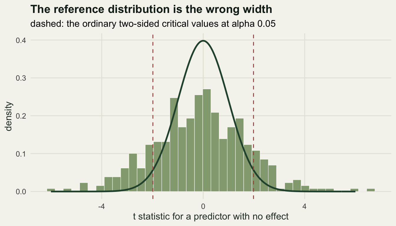
Why the permutation still sits above five per cent
MMRR is much better than the ordinary test and still not exact, and the reason is worth knowing before you quote a p just under 0.05. Permuting the raw response destroys every signal in it, including the real geographic effect. The permuted fits therefore have a larger residual variance than the observed fit, their t statistics are shrunk, and the observed t clears them too easily. That should make the inflation grow with the strength of the effect being kept in the model.
set.seed(2718)
sweep_tab <- do.call(rbind, lapply(c(0, 0.6, 1.2), function(bb) {
  st <- run_study(n_rep = 400, b1 = bb, b2 = 0)
  rr <- mean(st[, 3] < 0.05)
  data.frame(geographic_coefficient = bb,
             mmrr_rejection = round(rr, 4),
             mc_standard_error = round(sqrt(rr * (1 - rr) / 400), 4))
}))
print(sweep_tab, row.names = FALSE)
geographic_coefficient mmrr_rejection mc_standard_error
0.0 0.0650 0.0123
0.6 0.0875 0.0141
1.2 0.1225 0.0164With no geographic effect at all the permutation test is close to nominal, 0.0650 with a standard error of 0.0123. Add the effect and the false rejection rate climbs to 0.0875 and then 0.1225. So MMRR’s p-value is a good approximation when the model has little real signal in it and drifts anticonservative exactly when the analysis has something to report, which is the awkward direction. The published fix is to permute residuals under the reduced model rather than the raw response, and if a barrier effect matters to a conclusion at p near 0.05, that is the version to run.
Power, so the test is not merely cautious
A test that never rejects has a false positive rate of zero and is useless. Repeat the design with a genuine coefficient of 0.4 on the same spatially structured predictor.
set.seed(1618)
pow <- run_study(n_rep = 200, b1 = 0.6, b2 = 0.4)
pow_rate <- mean(pow[, 3] < 0.05)
cat("MMRR rejection rate with a true coefficient of 0.4:",
    round(pow_rate, 4), " Monte Carlo standard error:",
    round(sqrt(pow_rate * (1 - pow_rate) / 200), 4), "\n")
MMRR rejection rate with a true coefficient of 0.4: 0.745 Monte Carlo standard error: 0.0308 cat("ordinary lm rejection rate on the same replicates:",
round(mean(pow[, 1] < 0.05), 4), "\n")ordinary lm rejection rate on the same replicates: 0.91 cat("the same two rates as percentages:", round(100 * pow_rate, 2),
"and", round(100 * mean(pow[, 1] < 0.05), 2), "\n")the same two rates as percentages: 74.5 and 91 The permutation test finds the real effect 74.5 per cent of the time with 15 sites, against 91 per cent for the ordinary test, and the ordinary test buys that difference with a false positive rate of 26.75 per cent. Fifteen sites is a small landscape genetics study, and a power of 74.5 per cent for a moderate effect is a useful number to have before designing one.
What the test does not tell you
The permutation fixes the dependence between pairs and nothing else. It does not fix collinear predictor matrices: the two distances in the 18-site example correlated at 0.6481, and at that level the individual coefficients move a long way between datasets even when the test is valid. Two correlated candidate surfaces produce an unstable split of the same explained variation, which is the same problem as any collinear regression and is measured the same way, by the variance inflation factor.
The null being tested is “this predictor adds nothing once the others are in the model”. That is not “the landscape does not matter”. A resistance surface built with the wrong cost values, or the wrong transform from habitat to resistance, will fail this test while the landscape it was meant to describe matters a great deal. Failing to reject is a statement about one parameterisation, not about the biology.
And a permutation test is only as good as the exchangeability it assumes. Shuffling site labels assumes the sites are interchangeable under the null, which is false when the sampling design is clustered: a pair of sites in one valley and a distant third are not exchangeable, and permuting them builds null datasets that could not have arisen. That is a second source of trouble, and it is not the one measured above: the sites in this study are placed uniformly at random, so nothing here is clustered. The permutation test’s inflation came from permuting the raw response, and the ordinary test’s rate involves no permutation at all.
Where to go next
MMRR gives a defensible p-value for a surface you already have. It says nothing about whether that surface is the right one, and the type I error measured here is small compared with the freedom involved in choosing resistance values. The next tutorial in this cluster works through the checks a landscape genetics analysis needs before its coefficients mean anything: how many sites, how much collinearity is too much, what optimising a resistance surface does to the p-value that follows it, and how to tell a real barrier from a plausible-looking one.
References
Wang IJ 2013 Evolution 67(12):3403-3411 (10.1111/evo.12134)
Legendre P, Lapointe FJ, Casgrain P 1994 Evolution 48(5):1487-1499 (10.1111/j.1558-5646.1994.tb02191.x)
Guillot G, Rousset F 2013 Methods in Ecology and Evolution 4(4):336-344 (10.1111/2041-210X.12018)
Legendre P, Fortin MJ 2010 Molecular Ecology Resources 10(5):831-844 (10.1111/j.1755-0998.2010.02866.x)