library(ggplot2)

te_pal <- list(forest = "#275139", green = "#2f8f63", sage = "#93a87f",
               clay = "#b5534e", gold = "#cda23f", line = "#dad9ca",
               ink = "#16241d", paper = "#f5f4ee")

theme_te <- function() {
  theme_minimal(base_size = 12) +
    theme(panel.grid.minor = element_blank(),
          panel.grid.major = element_line(colour = "#e7e6dc"),
          plot.background = element_rect(fill = "#f5f4ee", colour = NA),
          panel.background = element_rect(fill = "#f5f4ee", colour = NA),
          plot.title = element_text(face = "bold", colour = te_pal$ink),
          axis.title = element_text(colour = "#2c3a31"))
}Isolation by distance and by resistance
R
landscape genetics
population genetics
ecology tutorial
ggplot2
Regress simulated genetic differentiation on Euclidean, least-cost and resistance distance in R, and see which of the three a barrier to gene flow shows up in.
Landscape genetics is mostly one regression. Take a genetic distance between every pair of sampled populations, take a between-site distance, and ask how much of the first the second explains. The interesting choice is not the statistic; it is which distance goes on the horizontal axis. Straight-line distance gives isolation by distance. Cost distance across a resistance surface gives the least-cost version. Effective resistance from circuit theory gives isolation by resistance.
This tutorial builds one lattice, lets gene flow happen on it, and then measures all three distances between the same fourteen sampled demes. Because the gene flow is simulated as a random walk on the conductance graph, the correct answer is known in advance, which makes the size of the differences between the three candidate distances the useful result rather than the ranking itself.
A lattice with a barrier
The landscape is a 20 by 20 grid of demes. Cell resistance comes from a smoothed random field, running from 1 in the best habitat to 60 in the most hostile, plus one hard feature: a two-cell-wide near-vertical band of resistance 1000 that steps sideways halfway down, with a single row left open. That gap is what makes the three distances disagree. Two demes on opposite sides of the band can be a handful of cells apart in a straight line and still exchange genes only by a long detour.
smooth_field <- function(n, passes, seed) {
  set.seed(seed)
  z <- matrix(runif(n * n), n, n)
  for (p in seq_len(passes)) {
    pad <- rbind(z[1, ], z, z[n, ])
    pad <- cbind(pad[, 1], pad, pad[, n])
    z <- (pad[1:n, 2:(n + 1)] + pad[3:(n + 2), 2:(n + 1)] +
            pad[2:(n + 1), 1:n] + pad[2:(n + 1), 3:(n + 2)] +
            4 * pad[2:(n + 1), 2:(n + 1)]) / 8
  }
  (z - min(z)) / (max(z) - min(z))
}

shift_mat <- function(m, dy, dx) {
  n <- nrow(m)
  nc <- ncol(m)
  out <- matrix(Inf, n, nc)
  yi <- max(1, 1 - dy):min(n, n - dy)
  xi <- max(1, 1 - dx):min(nc, nc - dx)
  out[yi, xi] <- m[yi + dy, xi + dx]
  out
}

cost_distance <- function(res, src, max_iter = 2000) {
  d <- matrix(Inf, nrow(res), ncol(res))
  d[src] <- 0
  moves <- list(c(-1, 0), c(1, 0), c(0, -1), c(0, 1))
  for (it in seq_len(max_iter)) {
    old <- d
    for (mv in moves) {
      d <- pmin(d, shift_mat(d, mv[1], mv[2]) +
                  (res + shift_mat(res, mv[1], mv[2])) / 2)
    }
    if (all(old == d)) break
  }
  d
}

build_laplacian <- function(res) {
  n <- nrow(res)
  nc <- ncol(res)
  ids <- matrix(seq_len(n * nc), n, nc)
  ii <- c(as.vector(ids[-n, ]), as.vector(ids[, -nc]))
  jj <- c(as.vector(ids[-1, ]), as.vector(ids[, -1]))
  cond <- 2 / (res[ii] + res[jj])
  lap <- matrix(0, n * nc, n * nc)
  lap[cbind(ii, jj)] <- -cond
  lap[cbind(jj, ii)] <- -cond
  diag(lap) <- -rowSums(lap)
  lap
}

resistance_all <- function(lap) {
  n_all <- nrow(lap)
  jm <- matrix(1 / n_all, n_all, n_all)
  lp <- solve(lap + jm) - jm
  dg <- diag(lp)
  outer(dg, dg, "+") - 2 * lp
}

effective_resistance <- function(lap, s, t_node) {
  n_all <- nrow(lap)
  cur <- numeric(n_all)
  cur[s] <- 1
  cur[t_node] <- -1
  keep <- setdiff(seq_len(n_all), t_node)
  v <- numeric(n_all)
  v[keep] <- solve(lap[keep, keep], cur[keep])
  v[s] - v[t_node]
}
resistance_all() is the only piece that is not a copy of the circuit tutorial. Ninety-one pairs would need ninety-one linear solves if each one grounded a different node. The pseudo-inverse of the Laplacian gives all of them at once, because R_ij = Lplus_ii + Lplus_jj - 2 Lplus_ij, and for a connected graph the pseudo-inverse is solve(L + J) - J with J the matrix of 1/n. One 400 by 400 solve replaces the loop.
n_side <- 20
quality <- smooth_field(n_side, 5, seed = 4821)
res_land <- 1 + 59 * (1 - quality)
gap_row <- 18
r_barrier <- 1000
for (rr in seq_len(n_side)) {
  band <- if (rr <= 10) c(10, 11) else c(11, 12)
  if (rr != gap_row) res_land[rr, band] <- r_barrier
}

cat("lattice:", n_side, "by", n_side, "=", n_side * n_side, "demes\n")
lattice: 20 by 20 = 400 demescat("habitat resistance range:",
round(range(res_land[res_land < r_barrier]), 2),
" barrier resistance:", r_barrier,
" barrier cells:", sum(res_land == r_barrier),
" open row in the barrier:", gap_row, "\n")habitat resistance range: 1 60 barrier resistance: 1000 barrier cells: 38 open row in the barrier: 18 Gene flow as a random walk on the conductance graph
Every cell is a Wright-Fisher deme of 50 diploids carrying 60 independent biallelic loci, all starting at a frequency of 0.5. One generation is two steps. First migration: each deme exchanges with its four rook neighbours at a rate proportional to the conductance 2 / (r_i + r_j), the same quantity the circuit solution uses, scaled so that the best connected cell sends out half of itself per generation. Then drift: 2N binomial draws per deme per locus.
Written as a weighted sum of shifted copies of the frequency matrix, the migration step is five multiplications on a 400 by 60 matrix, so 2500 generations of a 400-deme lattice takes a few seconds.
n_node <- n_side * n_side
ids <- matrix(seq_len(n_node), n_side, n_side)

neighbour_set <- function(dy, dx) {
  yy <- row(ids) + dy
  xx <- col(ids) + dx
  inside <- (yy >= 1) & (yy <= n_side) & (xx >= 1) & (xx <= n_side)
  list(id = as.vector(ids[cbind(as.vector(pmin(pmax(yy, 1), n_side)),
                                as.vector(pmin(pmax(xx, 1), n_side)))]),
       inside = as.vector(inside))
}

nbr <- lapply(list(c(-1, 0), c(1, 0), c(0, -1), c(0, 1)),
              function(v) neighbour_set(v[1], v[2]))
res_vec <- as.vector(res_land)
cond_dir <- lapply(nbr, function(b)
  ifelse(b$inside, 2 / (res_vec + res_vec[b$id]), 0))
cond_tot <- Reduce(`+`, cond_dir)
m_scale <- 0.5 / max(cond_tot)
mig_dir <- lapply(cond_dir, function(x) x * m_scale)
mig_stay <- 1 - cond_tot * m_scale
n_dip <- 50

cat("total emigration rate per deme: max", round(max(1 - mig_stay), 4),
    " mean", round(mean(1 - mig_stay), 4),
    " min", round(min(1 - mig_stay), 6), "\n")
total emigration rate per deme: max 0.5 mean 0.082 min 0.002034 cat("migrants per generation Nm: lattice mean",
round(n_dip * mean(1 - mig_stay), 3),
" most isolated deme", round(n_dip * min(1 - mig_stay), 4), "\n")migrants per generation Nm: lattice mean 4.098 most isolated deme 0.1017 The three printed rates are the whole model. The best connected deme replaces 0.5 of itself per generation, the lattice average is 0.082, and the most enclosed deme inside the barrier replaces 0.002034 of itself: a spread of more than two orders of magnitude, produced entirely by the resistance surface. The lattice mean number of migrants per generation is 4.098 while the most isolated deme receives 0.1017, so this is a weakly structured population with a few near-isolates in it, not a set of islands.
n_loci <- 60
gens <- 2500
cat("diploids per deme:", n_dip, " loci:", n_loci, " generations:", gens,
    " diploids on the lattice:", n_dip * n_node, "\n")
diploids per deme: 50 loci: 60 generations: 2500 diploids on the lattice: 20000 set.seed(4822)
p_frq <- matrix(0.5, n_node, n_loci)
for (g in seq_len(gens)) {
p_mig <- mig_stay * p_frq
for (k in seq_along(nbr)) p_mig <- p_mig + mig_dir[[k]] * p_frq[nbr[[k]]$id, ]
p_frq <- matrix(rbinom(length(p_mig), 2 * n_dip,
pmin(pmax(as.vector(p_mig), 0), 1)),
n_node, n_loci) / (2 * n_dip)
}
fixed_locus <- apply(p_frq, 2, function(x) max(x) < 1e-12 || min(x) > 1 - 1e-12)
p_keep <- p_frq[, !fixed_locus, drop = FALSE]
cat("loci monomorphic across the whole lattice:", sum(fixed_locus),
" loci kept:", ncol(p_keep), "\n")loci monomorphic across the whole lattice: 0 loci kept: 60 cat("lattice-wide allele frequency, range over kept loci:",
round(range(colMeans(p_keep)), 4), "\n")lattice-wide allele frequency, range over kept loci: 0.2649 0.7013 There is no mutation in this model, so allele frequencies are free to wander to fixation and any locus that gets there carries no information. After 2500 generations 0 of the 60 loci have gone monomorphic across the whole lattice, which is what should happen: the system holds 20000 diploids in total, and losing an allele from all of them takes far longer than losing it from one deme. Lattice-wide frequencies have drifted, from 0.2649 to 0.7013 across loci, but that drift is shared by every deme, so it adds no structure.
Fourteen demes, ninety-one pairs
Fourteen demes are sampled at fixed coordinates, seven on each side of the barrier, avoiding the barrier cells themselves. Pairwise Fst for each of the 91 pairs uses the two-population estimator summed over loci: Hs is the mean within-deme heterozygosity, Ht the heterozygosity of the pooled frequency, Fst = (Ht - Hs)/Ht. Following Rousset the quantity that should be linear in distance under a stepping-stone model is Fst/(1 - Fst), so that is what gets regressed.
sites <- data.frame(
  x = c(3, 7, 2, 6, 3, 8, 5, 15, 19, 14, 18, 15, 19, 16),
  y = c(2, 5, 9, 12, 16, 19, 8, 3, 6, 10, 13, 17, 20, 7))
sites$side <- ifelse(sites$x <= 10, "west", "east")
sites$node <- (sites$x - 1) * n_side + sites$y
prs <- t(combn(nrow(sites), 2))

pair_fst <- function(pa, pb) {
  p_bar <- (pa + pb) / 2
  hs <- (2 * pa * (1 - pa) + 2 * pb * (1 - pb)) / 2
  ht <- 2 * p_bar * (1 - p_bar)
  sum(ht - hs) / sum(ht)
}

gen <- data.frame(a = prs[, 1], b = prs[, 2])
gen$fst <- apply(prs, 1, function(k)
  pair_fst(p_keep[sites$node[k[1]], ], p_keep[sites$node[k[2]], ]))
gen$lin <- gen$fst / (1 - gen$fst)
gen$crosses <- sites$side[gen$a] != sites$side[gen$b]

cat("sampled demes:", nrow(sites), " west", sum(sites$side == "west"),
    " east", sum(sites$side == "east"), " pairs", nrow(gen),
    " crossing the barrier", sum(gen$crosses),
    " pairs containing any one deme:", nrow(sites) - 1, "\n")
sampled demes: 14 west 7 east 7 pairs 91 crossing the barrier 49 pairs containing any one deme: 13 cat("pairwise Fst: min", round(min(gen$fst), 4),
" median", round(median(gen$fst), 4),
" max", round(max(gen$fst), 4), "\n")pairwise Fst: min 0.0407 median 0.1011 max 0.1789 Now the three distances between the same fourteen points. Euclidean distance comes from the coordinates, least-cost distance from one sweep per site with the same edge cost convention the circuit uses (the mean of the two cell resistances), and resistance distance from the pseudo-inverse. The pseudo-inverse is worth checking against a single-pair solve before trusting 91 numbers from it.
gen$euclid <- sqrt((sites$x[gen$a] - sites$x[gen$b])^2 +
                     (sites$y[gen$a] - sites$y[gen$b])^2)

lcp_cols <- sapply(seq_len(nrow(sites)), function(k) {
  src <- matrix(FALSE, n_side, n_side)
  src[sites$y[k], sites$x[k]] <- TRUE
  cost_distance(res_land, src)[cbind(sites$y, sites$x)]
})
gen$leastcost <- lcp_cols[cbind(gen$a, gen$b)]

lap <- build_laplacian(res_land)
r_all <- resistance_all(lap)
gen$resist <- r_all[cbind(sites$node[gen$a], sites$node[gen$b])]

chk <- effective_resistance(lap, sites$node[1], sites$node[14])
r_absdiff <- signif(abs(r_all[sites$node[1], sites$node[14]] - chk), 3)
cat("resistance between sites 1 and 14: pseudo-inverse",
    round(r_all[sites$node[1], sites$node[14]], 6),
    " single-pair solve:", round(chk, 6),
    " absolute difference:",
    r_absdiff, "\n")
resistance between sites 1 and 14: pseudo-inverse 112.9407 single-pair solve: 112.9407 absolute difference: 1.54e-11 cat("Euclidean range:", round(range(gen$euclid), 2),
" least-cost range:", round(range(gen$leastcost), 1),
" resistance range:", round(range(gen$resist), 2), "\n")Euclidean range: 3.16 24.08 least-cost range: 57.5 935 resistance range: 17.59 131.88 The two routes to the same number agree, 112.9407 against 112.9407, with an absolute difference of 1.54e-11, which is solver noise rather than disagreement. Pairwise Fst runs from 0.0407 to 0.1789 with a median of 0.1011, the range a real microsatellite study on a fragmented species might report.
land_df <- data.frame(x = rep(seq_len(n_side), each = n_side),
                      y = rep(seq_len(n_side), times = n_side),
                      resistance = as.vector(res_land))

ggplot(land_df, aes(x, y)) +
  geom_raster(aes(fill = pmin(resistance, 60))) +
  geom_tile(data = subset(land_df, resistance > 60), fill = te_pal$ink) +
  geom_point(data = sites, aes(x, y), colour = "white", size = 4.2) +
  geom_point(data = sites, aes(x, y, colour = side), size = 2.6) +
  coord_equal() +
  scale_fill_gradient(low = te_pal$paper, high = te_pal$green,
                      name = "resistance") +
  scale_colour_manual(values = c(west = te_pal$gold, east = te_pal$clay),
                      name = "side") +
  labs(title = "One barrier with one gap",
       subtitle = "habitat resistance 1 to 60, barrier cells in black, row 18 open",
       x = NULL, y = NULL) +
  theme_te() +
  theme(panel.grid = element_blank())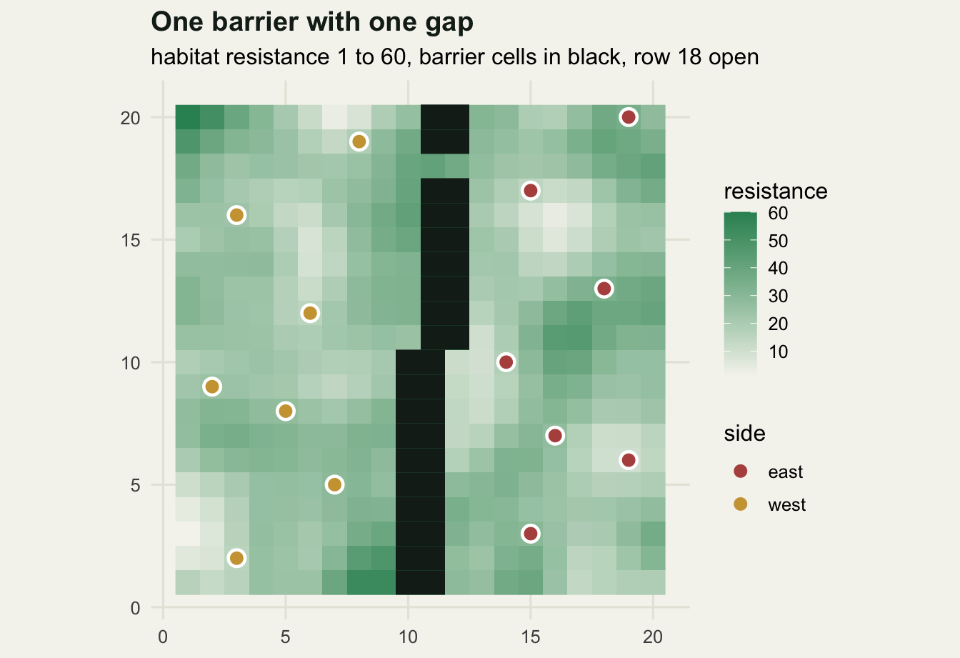
Which distance fits the genetic data?
metrics <- c("euclid", "leastcost", "resist")
fit_tab <- data.frame(
  distance = c("Euclidean", "least-cost", "resistance"),
  correlation = round(as.numeric(sapply(metrics, function(v)
    cor(gen[[v]], gen$lin))), 4),
  r_squared = round(as.numeric(sapply(metrics, function(v)
    summary(lm(gen$lin ~ gen[[v]]))$r.squared)), 4))
print(fit_tab, row.names = FALSE)
distance correlation r_squared
Euclidean 0.6303 0.3973
least-cost 0.8165 0.6666
resistance 0.7649 0.5850cat("correlations among the distances themselves: Euclidean and least-cost",
round(cor(gen$euclid, gen$leastcost), 4),
" Euclidean and resistance", round(cor(gen$euclid, gen$resist), 4),
" least-cost and resistance", round(cor(gen$leastcost, gen$resist), 4),
"\n")correlations among the distances themselves: Euclidean and least-cost 0.736 Euclidean and resistance 0.7745 least-cost and resistance 0.9251 The r squared against linearised Fst is 0.3973 for Euclidean distance, 0.6666 for least-cost distance and 0.5850 for resistance distance. A study that stopped at isolation by distance would have reported that geography explains the differentiation, and would have had no way to see what the barrier accounts for.
The ordering of the two landscape distances is the part not to over-read. Gene flow in this simulation is exactly a random walk on the conductance graph, which is the process effective resistance is derived from, and here it is least-cost distance that fits slightly better. The reason is in the second line of output: the two landscape distances correlate at 0.9251 with each other. When a hard barrier dominates the surface, cost distance becomes close to an indicator of whether the pair has to detour, and that indicator carries most of the signal a resistance distance carries. Ninety-one pairs cannot separate two predictors that similar.
long_names <- c(euclid = "Euclidean distance",
                leastcost = "Least-cost distance",
                resist = "Resistance distance")
fit_df <- do.call(rbind, lapply(metrics, function(v) {
  mod <- lm(gen$lin ~ gen[[v]])
  xs <- seq(min(gen[[v]]), max(gen[[v]]), length.out = 50)
  data.frame(distance = xs,
             lin = coef(mod)[[1]] + coef(mod)[[2]] * xs,
             panel = long_names[[v]])
}))
pts_df <- do.call(rbind, lapply(metrics, function(v)
  data.frame(distance = gen[[v]], lin = gen$lin,
             pair = ifelse(gen$crosses, "crosses the barrier", "same side"),
             panel = long_names[[v]])))

ggplot(pts_df, aes(distance, lin)) +
  geom_line(data = fit_df, colour = "grey45", linewidth = 0.8) +
  geom_point(aes(colour = pair), size = 1.9, alpha = 0.9) +
  facet_wrap(~panel, scales = "free_x") +
  scale_colour_manual(values = c(`crosses the barrier` = te_pal$clay,
                                 `same side` = te_pal$forest), name = NULL) +
  labs(title = "Same genetic data, three horizontal axes",
       subtitle = "91 pairs from 14 demes, grey line fitted to all pairs in the panel",
       x = "between-site distance", y = "Fst / (1 - Fst)") +
  theme_te() +
  theme(legend.position = "bottom")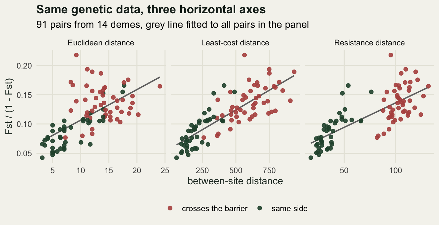
Where the metrics disagree: the barrier
The regression summaries hide what the landscape distances are picking up. Split the 91 pairs by whether they cross the barrier and compare them at Euclidean distances where both groups exist.
win_lo <- 8
win_hi <- 16
win <- gen$euclid >= win_lo & gen$euclid <= win_hi
cat("Euclidean window used for the matched comparison:", win_lo, "to", win_hi,
    "cells\n")
Euclidean window used for the matched comparison: 8 to 16 cellssplit_tab <- data.frame(
pairs = c("crossing the barrier", "same side"),
n = c(sum(win & gen$crosses), sum(win & !gen$crosses)),
mean_euclid = round(c(mean(gen$euclid[win & gen$crosses]),
mean(gen$euclid[win & !gen$crosses])), 2),
mean_resist = round(c(mean(gen$resist[win & gen$crosses]),
mean(gen$resist[win & !gen$crosses])), 1),
mean_lin_fst = round(c(mean(gen$lin[win & gen$crosses]),
mean(gen$lin[win & !gen$crosses])), 4))
print(split_tab, row.names = FALSE) pairs n mean_euclid mean_resist mean_lin_fst
crossing the barrier 34 12.42 101.1 0.1393
same side 14 11.87 47.2 0.1052cat("Euclidean distance, overlap of the two groups: barrier pairs from",
round(min(gen$euclid[gen$crosses]), 2), "and same-side pairs up to",
round(max(gen$euclid[!gen$crosses]), 2), "\n")Euclidean distance, overlap of the two groups: barrier pairs from 7.28 and same-side pairs up to 17.72 cat("resistance distance, same comparison: barrier pairs from",
round(min(gen$resist[gen$crosses]), 2), "and same-side pairs up to",
round(max(gen$resist[!gen$crosses]), 2), "\n")resistance distance, same comparison: barrier pairs from 81.92 and same-side pairs up to 76.33 res_e <- residuals(lm(lin ~ euclid, data = gen))
res_r <- residuals(lm(lin ~ resist, data = gen))
cat("mean residual from the Euclidean fit: barrier pairs",
round(mean(res_e[gen$crosses]), 4), " same side",
round(mean(res_e[!gen$crosses]), 4), "\n")mean residual from the Euclidean fit: barrier pairs 0.0093 same side -0.0108 cat("mean residual from the resistance fit: barrier pairs",
round(mean(res_r[gen$crosses]), 4), " same side",
round(mean(res_r[!gen$crosses]), 4), "\n")mean residual from the resistance fit: barrier pairs -0.0026 same side 0.0031 Between 8 and 16 cells apart there are 34 pairs separated by the barrier and 14 pairs on the same side, at almost the same mean Euclidean distance, 12.42 against 11.87. On this marker set their mean linearised Fst is 0.1393 and 0.1052: more differentiation for the same map distance. Their mean resistance distance is 101.1 against 47.2, which is where that difference comes from.
On the Euclidean axis the two groups are thoroughly mixed. Barrier pairs start at 7.28 cells and same-side pairs run up to 17.72, so no cut on straight-line distance separates them. On the resistance axis the separation is cleaner: the closest barrier pair sits at 81.92 and the most distant same-side pair at 76.33. The residuals say the same thing in the language of the regression. Fitting on Euclidean distance leaves the barrier pairs 0.0093 above the line on average and the same-side pairs 0.0108 below it, an offset in opposite directions for the two groups, which is what a missing predictor leaves behind when it is strong enough to show. Fitting on resistance distance leaves residuals of -0.0026 and 0.0031, smaller on this run and with the signs swapped: shrinking that offset is the entire point of a resistance surface, and the residual means are where you check whether it happened.
coll_df <- data.frame(euclid = gen$euclid, resist = gen$resist,
                      pair = ifelse(gen$crosses, "crosses the barrier",
                                    "same side"))

ggplot(coll_df, aes(euclid, resist, colour = pair)) +
  geom_point(size = 2.2, alpha = 0.9) +
  scale_colour_manual(values = c(`crosses the barrier` = te_pal$clay,
                                 `same side` = te_pal$forest), name = NULL) +
  labs(title = "The barrier is invisible on the horizontal axis",
       subtitle = "same 91 pairs, resistance distance against straight-line distance",
       x = "Euclidean distance in cells", y = "resistance distance") +
  theme_te() +
  theme(legend.position = "bottom")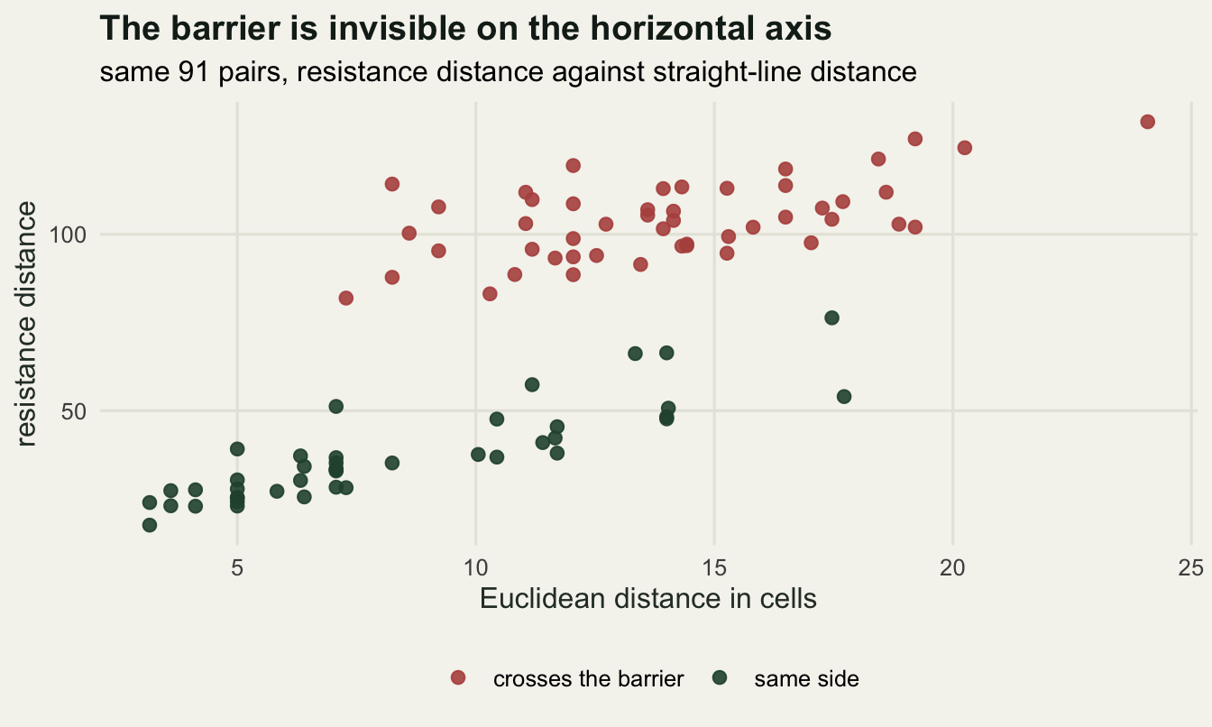
How stable is that ranking?
The full panel put both landscape distances ahead of Euclidean distance, with least-cost ahead of resistance, 0.6666 against 0.5850. Whether either ordering holds depends on the marker set. Split the loci into three disjoint blocks of 20 and recompute everything, holding the simulated history fixed and changing only which markers are read.
block_tab <- do.call(rbind, lapply(1:3, function(bk) {
  cols <- seq(bk, ncol(p_keep), by = 3)
  p_sub <- p_keep[, cols, drop = FALSE]
  fst_b <- apply(prs, 1, function(k)
    pair_fst(p_sub[sites$node[k[1]], ], p_sub[sites$node[k[2]], ]))
  lin_b <- fst_b / (1 - fst_b)
  data.frame(block = bk, loci = length(cols),
             euclidean = round(summary(lm(lin_b ~ gen$euclid))$r.squared, 4),
             least_cost = round(summary(lm(lin_b ~ gen$leastcost))$r.squared, 4),
             resistance = round(summary(lm(lin_b ~ gen$resist))$r.squared, 4))
}))
print(block_tab, row.names = FALSE)
block loci euclidean least_cost resistance
1 20 0.2824 0.4976 0.4996
2 20 0.2979 0.3906 0.2732
3 20 0.2321 0.4439 0.3858Least-cost distance beats Euclidean distance in all three blocks of this split: 0.4976 against 0.2824, 0.3906 against 0.2979, 0.4439 against 0.2321. Resistance distance does not. In the second block it explains 0.2732 against Euclidean 0.2979, so with twenty markers the comparison that looked decisive on the full panel can invert. The two landscape distances also swap places on this run: resistance is marginally ahead in the first block, 0.4996 against 0.4976, and clearly behind in the second. Twenty markers is few, but it is what a microsatellite panel gives, and this resamples only the loci, with the simulated history held fixed. A real study resamples both.
What this does not tell you
Three limits, in order of how often they are ignored.
The first is the one the table above makes concrete. Three strongly correlated predictors were compared on the same 91 points, and the model that generated the data was known to be a random walk on the conductance graph, yet the best fitting distance was not the one derived from that walk. A difference in r squared between two candidate distances is not evidence about the mechanism of gene flow. It is evidence that one predictor happens to line up slightly better with this realisation of the process, and the honest report of a model selection exercise on collinear distances is the spread, not the winner.
The second is about the sample size. There are 91 pairs but only 14 demes, and every deme appears in 13 of the pairs, so the pairs share information heavily and are nothing like 91 independent observations. That is why nothing above is a significance test and why no p-value appears anywhere in this post: the ordinary regression standard errors would be far too small, and the correct machinery is a permutation that shuffles demes rather than pairs. That is the next tutorial.
The third is about time. Every Fst here assumes the drift and migration balance has had time to settle at the spatial scale being measured, and this simulation ran 2500 generations to make sure it had. A barrier built a few dozen generations ago leaves no genetic signal yet, and one removed a few dozen generations ago still shows. The Fst value contains no clock, so a resistance surface fitted to genetic data describes a landscape from some number of generations ago, and finding out which number takes a separate experiment.
Where to go next
Three tutorials follow this one. The first replaces the single regression with multiple matrix regression, which puts several distances in one model and gets its significance from permuting the distance matrices rather than the pairs. The second treats the resistance surface as unknown and optimises its parameters against the genetic data, which is where landscape genetics stops being a comparison of two candidate maps. The third is the checking tutorial for the whole cluster: how much data a usable answer needs, what collinearity does to the parameter estimates, and how long a landscape feature has to have existed before the genetics can see it.
References
McRae BH 2006 Evolution 60(8):1551-1561 (10.1111/j.0014-3820.2006.tb00500.x)
McRae BH, Beier P 2007 Proceedings of the National Academy of Sciences 104(50):19885-19890 (10.1073/pnas.0706568104)
Rousset F 1997 Genetics 145(4):1219-1228 (10.1093/genetics/145.4.1219)
Slatkin M 1993 Evolution 47(1):264-279 (10.1111/j.1558-5646.1993.tb01215.x)
Spear SF, Balkenhol N, Fortin MJ, McRae BH, Scribner KT 2010 Molecular Ecology 19(17):3576-3591 (10.1111/j.1365-294X.2010.04657.x)