library(ggplot2)

te_pal <- list(forest = "#275139", green = "#2f8f63", sage = "#93a87f",
               clay = "#b5534e", gold = "#cda23f", line = "#dad9ca",
               ink = "#16241d", paper = "#f5f4ee")

theme_te <- function() {
  theme_minimal(base_size = 12) +
    theme(panel.grid.minor = element_blank(),
          panel.grid.major = element_line(colour = "#e7e6dc"),
          plot.background = element_rect(fill = "#f5f4ee", colour = NA),
          panel.background = element_rect(fill = "#f5f4ee", colour = NA),
          plot.title = element_text(face = "bold", colour = te_pal$ink),
          axis.title = element_text(colour = "#2c3a31"))
}Circuit theory and effective resistance
R
landscape ecology
GIS
ecology tutorial
ggplot2
Solve a landscape as an electrical circuit in base R, map current density, and measure the thing least-cost paths cannot see: whether a redundant route exists.
Corrected 7 October 2026: the captions of both current maps did not say that their colour scales are capped; they now say that the cells carrying the most current take the end colour and so look less extreme than they are.
A least-cost path assumes the walker knows the whole landscape and takes the single best route. Circuit theory assumes the opposite: the walker moves at random, biased only locally by how easy each step is. Both are caricatures, and the difference between them is exactly the quantity that matters most for planning, because only one of them notices whether an alternative route exists.
This tutorial treats the landscape as a resistor network, solves it with the graph Laplacian in base R, and measures the redundancy effect that gives circuit theory its reputation.
The landscape as a circuit
Every cell is a node, adjacent cells are joined by a resistor whose resistance is the mean of the two cell resistances, and connectivity is measured by injecting one unit of current at the source and extracting it at the destination. The voltage difference that appears between them is the effective resistance, and the current flowing through each cell is the current density map.
build_laplacian <- function(res) {
  n <- nrow(res)
  m <- ncol(res)
  idx <- matrix(seq_len(n * m), n, m)
  ii <- c(as.vector(idx[-n, ]), as.vector(idx[, -m]))
  jj <- c(as.vector(idx[-1, ]), as.vector(idx[, -1]))
  cond <- 2 / (res[ii] + res[jj])
  lap <- matrix(0, n * m, n * m)
  for (k in seq_along(ii)) {
    lap[ii[k], jj[k]] <- lap[ii[k], jj[k]] - cond[k]
    lap[jj[k], ii[k]] <- lap[jj[k], ii[k]] - cond[k]
    lap[ii[k], ii[k]] <- lap[ii[k], ii[k]] + cond[k]
    lap[jj[k], jj[k]] <- lap[jj[k], jj[k]] + cond[k]
  }
  list(lap = lap, ii = ii, jj = jj, cond = cond)
}

effective_resistance <- function(res, s, t_node) {
  g <- build_laplacian(res)
  n_all <- nrow(g$lap)
  cur <- numeric(n_all)
  cur[s] <- 1
  cur[t_node] <- -1
  keep <- setdiff(seq_len(n_all), t_node)
  v <- numeric(n_all)
  v[keep] <- solve(g$lap[keep, keep], cur[keep])
  edge_cur <- g$cond * abs(v[g$ii] - v[g$jj])
  dens <- numeric(n_all)
  for (k in seq_along(edge_cur)) {
    dens[g$ii[k]] <- dens[g$ii[k]] + edge_cur[k] / 2
    dens[g$jj[k]] <- dens[g$jj[k]] + edge_cur[k] / 2
  }
  list(r_eff = v[s] - v[t_node], density = dens)
}

shift_mat <- function(m, dy, dx) {
  n <- nrow(m)
  p <- ncol(m)
  out <- matrix(Inf, n, p)
  yi <- max(1, 1 - dy):min(n, n - dy)
  xi <- max(1, 1 - dx):min(p, p - dx)
  out[yi, xi] <- m[yi + dy, xi + dx]
  out
}

cost_distance <- function(res, src, max_iter = 4000) {
  d <- matrix(Inf, nrow(res), ncol(res))
  d[src] <- 0
  moves <- list(c(-1, 0), c(1, 0), c(0, -1), c(0, 1))
  for (it in seq_len(max_iter)) {
    old <- d
    for (mv in moves) {
      d <- pmin(d, shift_mat(d, mv[1], mv[2]) +
                  (res + shift_mat(res, mv[1], mv[2])) / 2)
    }
    if (all(old == d)) break
  }
  d
}
Grounding one node before solving is not optional: the Laplacian is singular because voltages are only defined up to a constant, so the destination node is dropped from the system and its voltage set to zero. Dense solve() is fine at this grid size and keeps the code readable; a real analysis on a large raster needs a sparse solver.
The experiment least-cost paths fail
Build a landscape in which the matrix is expensive and one cheap corridor runs north to south, plus cheap bands along the top and bottom edges so that both ends are reachable. Then add a second, identical corridor and recompute both metrics.
n <- 41
one <- matrix(200, n, n)
one[, 11:13] <- 1
one[1:3, ] <- 1
one[(n - 2):n, ] <- 1
two <- one
two[, 29:31] <- 1

s_node <- 2 + (2 - 1) * n
t_node <- (n - 1) + (n - 1 - 1) * n

report <- function(res, nm) {
  src <- matrix(FALSE, n, n)
  src[((s_node - 1) %% n) + 1, ((s_node - 1) %/% n) + 1] <- TRUE
  d <- cost_distance(res, src)
  e <- effective_resistance(res, s_node, t_node)
  data.frame(landscape = nm,
             least_cost = round(d[((t_node - 1) %% n) + 1,
                                  ((t_node - 1) %/% n) + 1], 2),
             effective_resistance = round(e$r_eff, 4))
}

tab_a <- rbind(report(one, "one corridor"), report(two, "two corridors"))
print(tab_a, row.names = FALSE)
landscape least_cost effective_resistance
one corridor 76 23.3430
two corridors 76 15.3952cat("ratio of effective resistances:",
round(tab_a$effective_resistance[1] / tab_a$effective_resistance[2], 4),
" ratio of least-cost distances:",
round(tab_a$least_cost[1] / tab_a$least_cost[2], 4), "\n")ratio of effective resistances: 1.5163 ratio of least-cost distances: 1 The least-cost distance is 76 in both landscapes, identical to the digit, because the cheapest route is still one corridor and a second copy of it changes nothing about the best route. Effective resistance falls from 23.343 to 15.3952, a ratio of 1.5163.
That ratio is worth understanding rather than just quoting. Two identical parallel resistors halve the resistance, so a naive expectation is 2. The measured value is lower because the two corridors share the cheap bands at the top and bottom: those segments are in series with the parallel part, and series resistance does not halve. The point stands in the direction that matters: duplicating a route leaves the least-cost metric completely blind and moves the circuit metric by a third.
For conservation planning this is the whole argument for circuit theory. A landscape with two independent routes survives the loss of either one, and a metric that cannot see the difference will rate a fragile single-corridor network as highly as a redundant one.
dens_df <- do.call(rbind, lapply(list(list(one, "one corridor"),
                                      list(two, "two corridors")),
                                 function(z) {
  e <- effective_resistance(z[[1]], s_node, t_node)
  data.frame(x = rep(seq_len(n), each = n), y = rep(seq_len(n), times = n),
             current = e$density, panel = z[[2]])
}))

ggplot(dens_df, aes(x, y, fill = pmin(current, quantile(current, 0.995)))) +
  geom_raster() +
  facet_wrap(~panel) +
  coord_equal() +
  scale_fill_gradient(low = te_pal$paper, high = te_pal$forest,
                      name = "current") +
  labs(title = "A second corridor splits the current",
       subtitle = "same endpoints, same least-cost distance of 76",
       x = NULL, y = NULL) +
  theme_te() +
  theme(axis.text = element_blank(), panel.grid = element_blank())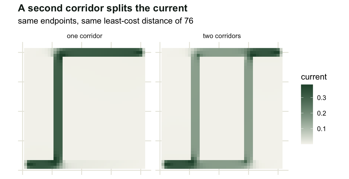
On a real-looking surface
Synthetic corridors make the point cleanly; a continuous resistance surface is what an analysis actually gets. Solve the same circuit on a smoothly varying surface and compare the current map with the least-cost corridor from the previous tutorial.
smooth_field <- function(n, passes, seed) {
  set.seed(seed)
  z <- matrix(runif(n * n), n, n)
  for (p in seq_len(passes)) {
    pad <- rbind(z[1, ], z, z[n, ])
    pad <- cbind(pad[, 1], pad, pad[, n])
    z <- (pad[1:n, 2:(n + 1)] + pad[3:(n + 2), 2:(n + 1)] +
            pad[2:(n + 1), 1:n] + pad[2:(n + 1), 3:(n + 2)] +
            4 * pad[2:(n + 1), 2:(n + 1)]) / 8
  }
  (z - min(z)) / (max(z) - min(z))
}

nn <- 41
qual <- smooth_field(nn, 6, seed = 474)
res_b <- 1 + 99 * (1 - qual)
s2 <- 4 + (4 - 1) * nn
t2 <- (nn - 3) + (nn - 3 - 1) * nn
e2 <- effective_resistance(res_b, s2, t2)

src2 <- matrix(FALSE, nn, nn)
src2[4, 4] <- TRUE
snk2 <- matrix(FALSE, nn, nn)
snk2[nn - 3, nn - 3] <- TRUE
corr <- cost_distance(res_b, src2) + cost_distance(res_b, snk2)
dens <- matrix(e2$density, nn, nn)
ord <- order(dens, decreasing = TRUE)

cat("effective resistance:", round(e2$r_eff, 4), "\n")
effective resistance: 142.7975 cat("share of current in the top 5 per cent of cells:",
round(sum(dens[ord[seq_len(round(0.05 * nn * nn))]]) / sum(dens), 4),
" in the top 20 per cent:",
round(sum(dens[ord[seq_len(round(0.2 * nn * nn))]]) / sum(dens), 4), "\n")share of current in the top 5 per cent of cells: 0.1609 in the top 20 per cent: 0.4179 cat("least-cost corridor within five per cent of the minimum covers:",
round(mean(corr <= 1.05 * min(corr)), 4), "of the map\n")least-cost corridor within five per cent of the minimum covers: 0.2118 of the mapcat("Spearman correlation, current density against negative corridor cost:",
round(cor(as.vector(dens), -as.vector(corr), method = "spearman"), 4), "\n")Spearman correlation, current density against negative corridor cost: 0.8007 The two models mostly agree: the rank correlation between current density and the least-cost corridor surface is 0.8007, so cells that carry current are largely the cells the corridor analysis would highlight. Where they differ is concentration. The top five per cent of cells carry only 16.09 per cent of the current and the top fifth carries 41.79 per cent, so on a smooth surface the current spreads out rather than funnelling.
That is a useful corrective to the language of pinch points. Pinch points are real where the landscape has few alternatives, which is the synthetic corridor case; on a gently varying surface, the current density map is broad, and picking its top few per cent as “the corridor” imposes a sharpness the model does not contain.
surf_df <- data.frame(x = rep(seq_len(nn), each = nn),
                      y = rep(seq_len(nn), times = nn),
                      current = as.vector(dens),
                      corridor = as.vector(corr <= 1.05 * min(corr)))

ggplot(surf_df, aes(x, y)) +
  geom_raster(aes(fill = pmin(current, quantile(current, 0.99)))) +
  geom_contour(aes(z = as.numeric(corridor)), breaks = 0.5,
               colour = te_pal$clay, linetype = "dashed", linewidth = 0.6) +
  coord_equal() +
  scale_fill_gradient(low = te_pal$paper, high = te_pal$forest,
                      name = "current") +
  labs(title = "Current spreads where alternatives exist",
       subtitle = "dashed: least-cost corridor within five per cent of the cheapest total cost",
       x = NULL, y = NULL) +
  theme_te() +
  theme(axis.text = element_blank(), panel.grid = element_blank())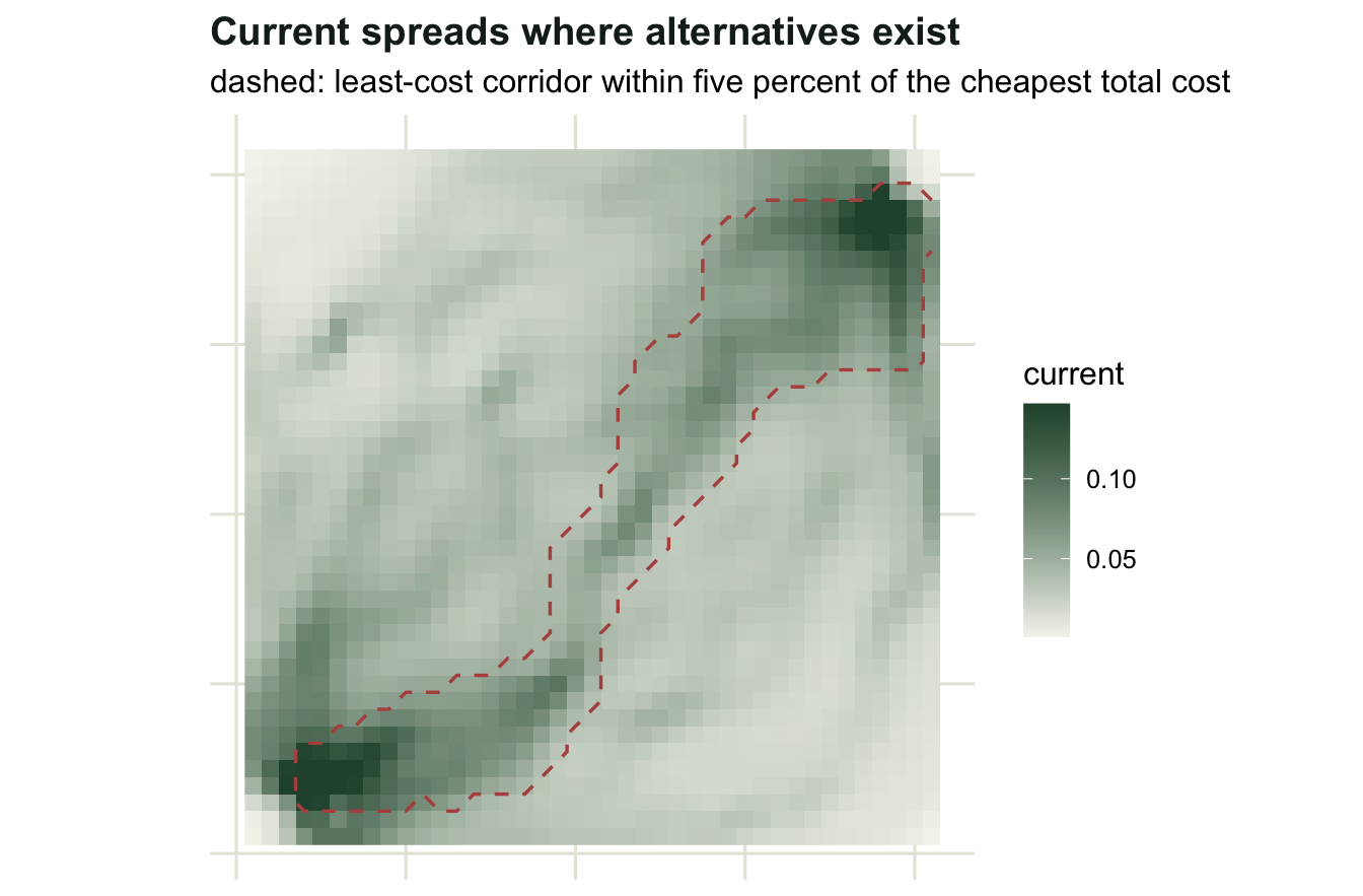
Which metric, and for what
Three practical distinctions come out of the measurements.
Effective resistance answers “how well connected are these two places, counting every route”, so it is the metric to use when the question is about redundancy, when several routes plausibly exist, or when a genetic distance is the response variable, because a random walk is a better caricature of gene flow over many generations than an optimal path is.
Least-cost distance answers “what is the best single route”, which is the right question for a planned intervention: a wildlife crossing, a hedgerow, a corridor purchase. It is also cheaper to compute and easier to explain.
Neither is a movement model. Both ignore behaviour, mortality risk, memory, and the fact that dispersers often cross hostile ground fast rather than avoiding it. The next tutorial makes that comparison quantitative by computing the expected time a random walker actually takes, and asking which of the three distances predicts it.
References
McRae BH 2006 Evolution 60(8):1551-1561 (10.1111/j.0014-3820.2006.tb00500.x)
McRae BH, Dickson BG, Keitt TH, Shah VB 2008 Ecology 89(10):2712-2724 (10.1890/07-1861.1)
Chandra AK, Raghavan P, Ruzzo WL, Smolensky R, Tiwari P 1996 Computational Complexity 6(4):312-340 (10.1007/BF01270385)