Checking a connectivity analysis

Four checks for a resistance-surface analysis in R: calibrate the metric, test what it predicts, vary the transform, and change the grain before believing it.

A connectivity analysis produces a map, and maps are persuasive. The three tutorials before this one built the pieces; this one asks what would have to be true for the output to mean anything, and measures each condition on simulated landscapes where the answer is known.

Four checks: calibrate the metric against the process it claims to summarise, test what it actually predicts, vary the arbitrary parts, and change the grain.

library(ggplot2)

te_pal <- list(forest = "#275139", green = "#2f8f63", sage = "#93a87f",
               clay = "#b5534e", gold = "#cda23f", line = "#dad9ca",
               ink = "#16241d", paper = "#f5f4ee")

theme_te <- function() {
  theme_minimal(base_size = 12) +
    theme(panel.grid.minor = element_blank(),
          panel.grid.major = element_line(colour = "#e7e6dc"),
          plot.background = element_rect(fill = "white", colour = NA),
          panel.background = element_rect(fill = "white", colour = NA),
          plot.title = element_text(face = "bold", colour = te_pal$ink),
          axis.title = element_text(colour = "#2c3a31"))
}

smooth_field <- function(n, passes, seed) {
  set.seed(seed)
  z <- matrix(runif(n * n), n, n)
  for (p in seq_len(passes)) {
    pad <- rbind(z[1, ], z, z[n, ])
    pad <- cbind(pad[, 1], pad, pad[, n])
    z <- (pad[1:n, 2:(n + 1)] + pad[3:(n + 2), 2:(n + 1)] +
            pad[2:(n + 1), 1:n] + pad[2:(n + 1), 3:(n + 2)] +
            4 * pad[2:(n + 1), 2:(n + 1)]) / 8
  }
  (z - min(z)) / (max(z) - min(z))
}

build_laplacian <- function(res) {
  n <- nrow(res)
  m <- ncol(res)
  idx <- matrix(seq_len(n * m), n, m)
  ii <- c(as.vector(idx[-n, ]), as.vector(idx[, -m]))
  jj <- c(as.vector(idx[-1, ]), as.vector(idx[, -1]))
  cond <- 2 / (res[ii] + res[jj])
  lap <- matrix(0, n * m, n * m)
  for (k in seq_along(ii)) {
    lap[ii[k], jj[k]] <- lap[ii[k], jj[k]] - cond[k]
    lap[jj[k], ii[k]] <- lap[jj[k], ii[k]] - cond[k]
    lap[ii[k], ii[k]] <- lap[ii[k], ii[k]] + cond[k]
    lap[jj[k], jj[k]] <- lap[jj[k], jj[k]] + cond[k]
  }
  lap
}

resistance_kit <- function(res) {
  lap <- build_laplacian(res)
  ground <- nrow(lap)
  list(inv = solve(lap[-ground, -ground]), ground = ground,
       m2 = sum(diag(lap)))
}

r_eff_pair <- function(kit, i, j) {
  gr <- kit$ground
  f <- function(x) if (x > gr) x - 1 else x
  if (i == gr) return(kit$inv[f(j), f(j)])
  if (j == gr) return(kit$inv[f(i), f(i)])
  kit$inv[f(i), f(i)] + kit$inv[f(j), f(j)] - 2 * kit$inv[f(i), f(j)]
}

hitting_times <- function(res, target) {
  lap <- build_laplacian(res)
  n_all <- nrow(lap)
  prob <- -lap
  diag(prob) <- 0
  prob <- prob / diag(lap)
  keep <- setdiff(seq_len(n_all), target)
  h <- numeric(n_all)
  h[keep] <- solve(diag(length(keep)) - prob[keep, keep], rep(1, length(keep)))
  h
}

shift_mat <- function(m, dy, dx) {
  n <- nrow(m)
  p <- ncol(m)
  out <- matrix(Inf, n, p)
  yi <- max(1, 1 - dy):min(n, n - dy)
  xi <- max(1, 1 - dx):min(p, p - dx)
  out[yi, xi] <- m[yi + dy, xi + dx]
  out
}

cost_distance <- function(res, src, max_iter = 4000) {
  d <- matrix(Inf, nrow(res), ncol(res))
  d[src] <- 0
  moves <- list(c(-1, 0), c(1, 0), c(0, -1), c(0, 1))
  for (it in seq_len(max_iter)) {
    old <- d
    for (mv in moves) {
      d <- pmin(d, shift_mat(d, mv[1], mv[2]) +
                  (res + shift_mat(res, mv[1], mv[2])) / 2)
    }
    if (all(old == d)) break
  }
  d
}

Computing effective resistance for many pairs one solve at a time is wasteful. Grounding one node and inverting the reduced Laplacian once gives every pairwise resistance from three entries of that inverse, which turns twenty pairs into one matrix inversion.

Check 1: calibrate the metric against its own process

Effective resistance is advertised as the connectivity metric that corresponds to random-walk movement. There is an exact statement behind that: the commute time between two nodes, the expected number of steps to go and come back, equals the resistance times the sum of all node degrees. Before interpreting anything, check that the implementation satisfies it.

n <- 41
qual <- smooth_field(n, 6, seed = 475)
res_lin <- 1 + 99 * (1 - qual)
target <- (n - 3) + (n - 3 - 1) * n

set.seed(476)
sources <- sample(setdiff(seq_len(n * n), target), 20)
xy <- function(idx) cbind(((idx - 1) %% n) + 1, ((idx - 1) %/% n) + 1)
tgt_xy <- xy(target)
src_xy <- xy(sources)

kit <- resistance_kit(res_lin)
h_to <- hitting_times(res_lin, target)
one <- sources[1]
h_back <- hitting_times(res_lin, one)
commute <- h_to[one] + h_back[target]

cat("commute time from the random walk:", round(commute, 3), "\n")

commute time from the random walk: 18945.14 

cat("2m times effective resistance:",
    round(kit$m2 * r_eff_pair(kit, one, target), 3),
    " ratio:", round(commute / (kit$m2 * r_eff_pair(kit, one, target)), 6), "\n")

2m times effective resistance: 18945.14  ratio: 1 

The two numbers agree exactly, 18945.14 both ways, with a ratio of 1. That single line is worth writing in any analysis that uses resistance distance, because it validates two independent pieces of machinery at once: the circuit solution and the walk. If it fails, one of them is wrong, and no amount of interpretation will fix it.

Check 2: what does the metric predict?

The calibration also warns about something. Commute time is a round trip. A dispersing individual makes a one-way journey, and the expected one-way time is a different quantity. Compare all three distances against the expected one-way travel time of a random walker.

euclid <- sqrt(rowSums((src_xy -
                          matrix(tgt_xy, nrow(src_xy), 2, byrow = TRUE))^2))
snk <- matrix(FALSE, n, n)
snk[tgt_xy[1], tgt_xy[2]] <- TRUE
lcp <- cost_distance(res_lin, snk)[src_xy]
r_eff <- sapply(sources, function(s) r_eff_pair(kit, s, target))
hit <- h_to[sources]

sp <- function(a, b) round(cor(a, b, method = "spearman"), 4)
cat("rank correlation with one-way hitting time: Euclidean", sp(euclid, hit),
    " least-cost", sp(lcp, hit), " resistance", sp(r_eff, hit), "\n")

rank correlation with one-way hitting time: Euclidean 0.9202  least-cost 0.8436  resistance 0.4617 

cat("among the metrics: Euclidean and least-cost", sp(euclid, lcp),
    " Euclidean and resistance", sp(euclid, r_eff),
    " least-cost and resistance", sp(lcp, r_eff), "\n")

among the metrics: Euclidean and least-cost 0.9248  Euclidean and resistance 0.6614  least-cost and resistance 0.7353 

On this landscape, plain Euclidean distance predicts one-way travel time best (0.9202), least-cost distance is close behind (0.8436), and resistance distance is the weakest of the three (0.4617). That is not a strike against circuit theory; it is a statement about which question each metric answers. Resistance distance summarises the whole two-way flow between two places, which is the right analogue for gene flow accumulated over generations, and a poor analogue for how long one animal takes to arrive.

The second line is the awkward one for validation studies. The three metrics correlate with each other at 0.9248, 0.6614 and 0.7353, so they are not interchangeable, but Euclidean distance is nearly as good a predictor as the expensive metrics on this surface. A resistance surface earns its place only when it beats straight-line distance on independent data, and that comparison is the minimum bar for any connectivity paper.

pred_df <- rbind(
  data.frame(distance = euclid, hit = hit,
             metric = sprintf("Euclidean (rho %.2f)", sp(euclid, hit))),
  data.frame(distance = lcp, hit = hit,
             metric = sprintf("least-cost (rho %.2f)", sp(lcp, hit))),
  data.frame(distance = r_eff, hit = hit,
             metric = sprintf("resistance (rho %.2f)", sp(r_eff, hit))))

ggplot(pred_df, aes(distance, hit)) +
  geom_point(colour = te_pal$forest, size = 2) +
  facet_wrap(~metric, scales = "free_x") +
  scale_x_log10() +
  scale_y_log10() +
  labs(title = "Which distance predicts the walk?",
       subtitle = "expected one-way hitting time, twenty sources to one target",
       x = "distance metric (log scale)",
       y = "expected steps (log scale)") +
  theme_te()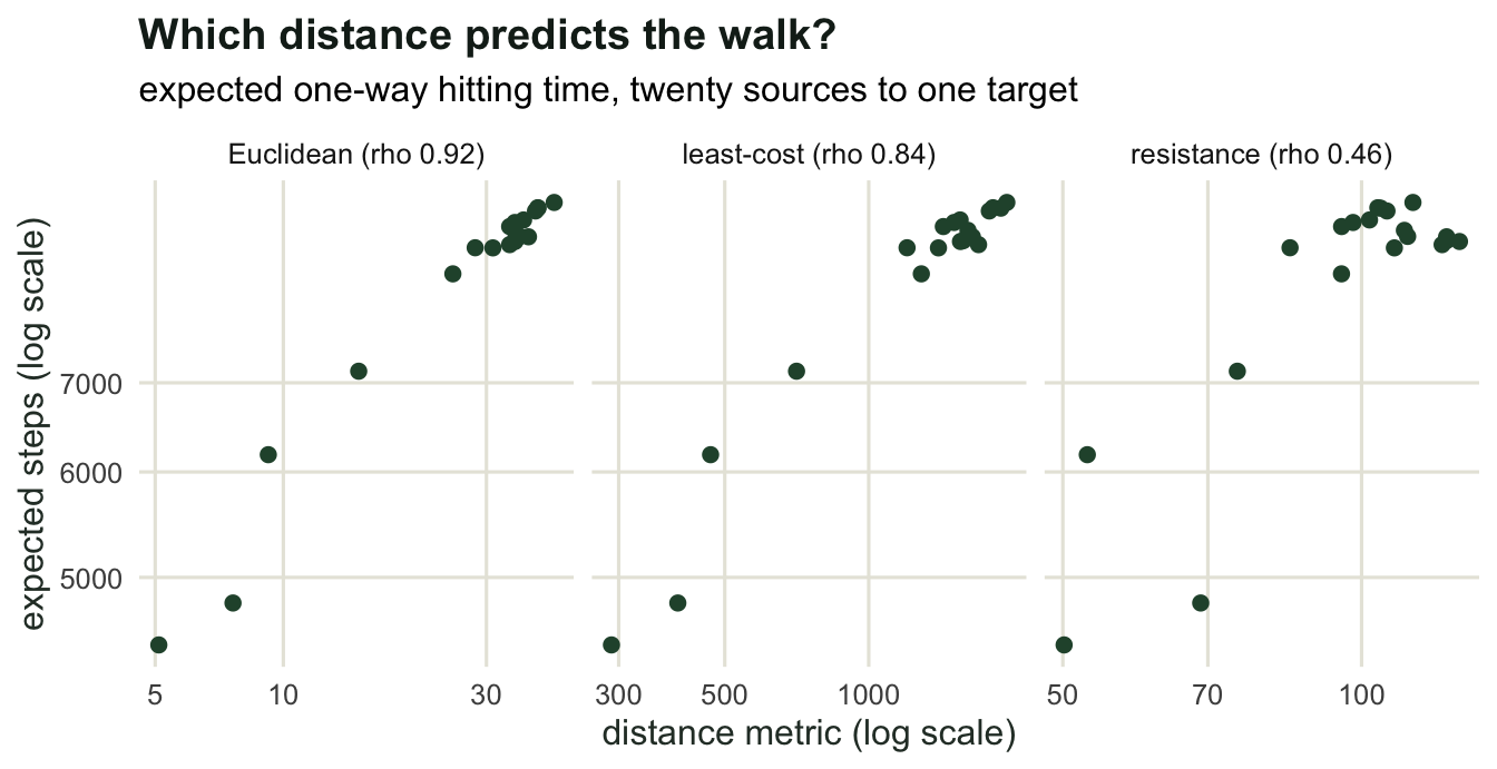

Figure 1: Expected one-way travel time of a random walker against three distance metrics, twenty source cells to one target, on log axes.

Check 3: vary the arbitrary part

Resistance values are assigned, not measured. The habitat quality surface can stay fixed while the transform from quality to resistance changes, and if the conclusions move, the conclusions were about the transform.

transforms <- list(linear = function(q) 1 + 99 * (1 - q),
                   exponential = function(q) exp(5 * (1 - q)),
                   threshold = function(q) ifelse(q > 0.5, 1, 100),
                   inverse = function(q) 1 / pmax(q, 0.01))

lcp_sets <- lapply(transforms, function(f) cost_distance(f(qual), snk)[src_xy])
reff_sets <- lapply(transforms, function(f) {
  k <- resistance_kit(f(qual))
  sapply(sources, function(s) r_eff_pair(k, s, target))
})

nms <- names(transforms)
trans_tab <- NULL
for (i in 1:3) {
  for (j in (i + 1):4) {
    trans_tab <- rbind(trans_tab, data.frame(
      pair = paste(nms[i], "vs", nms[j]),
      least_cost = sp(lcp_sets[[i]], lcp_sets[[j]]),
      resistance = sp(reff_sets[[i]], reff_sets[[j]])))
  }
}
print(trans_tab, row.names = FALSE)

                     pair least_cost resistance
    linear vs exponential     0.9398     0.9835
      linear vs threshold     0.5910     0.7714
        linear vs inverse     0.9188     0.9895
 exponential vs threshold     0.6887     0.7910
   exponential vs inverse     0.8301     0.9835
     threshold vs inverse     0.4286     0.7564

Two transforms that look similar can rank the same twenty pairs quite differently. Linear against exponential is safe (0.9398 for least-cost distance), but anything involving the threshold transform is not: linear against threshold gives 0.591 and threshold against inverse 0.4286. Effective resistance is consistently more stable across transforms (0.9835, 0.7714, 0.9895 and so on), because it integrates over the whole surface instead of following one route through it.

The practical rule: thresholding a continuous habitat surface into “habitat” and “matrix” is the single most consequential choice in a connectivity analysis, and it deserves an explicit sensitivity analysis rather than a sentence in the methods.

long_tab <- rbind(
  data.frame(pair = trans_tab$pair, value = trans_tab$least_cost,
             metric = "least-cost"),
  data.frame(pair = trans_tab$pair, value = trans_tab$resistance,
             metric = "resistance"))
long_tab$pair <- factor(long_tab$pair, levels = trans_tab$pair)

ggplot(long_tab, aes(pair, value, fill = metric)) +
  geom_col(position = position_dodge(width = 0.75), width = 0.65,
           colour = "white") +
  scale_fill_manual(values = c(`least-cost` = te_pal$clay,
                               resistance = te_pal$forest), name = NULL) +
  coord_cartesian(ylim = c(0, 1)) +
  labs(title = "How much does the transform decide?",
       subtitle = "rank correlation of the same twenty pairwise distances",
       x = NULL, y = "Spearman correlation") +
  theme_te() +
  theme(axis.text.x = element_text(angle = 20, hjust = 1))

Figure 2: Rank correlation of the twenty pairwise distances between resistance transforms, for least-cost distance and for effective resistance.

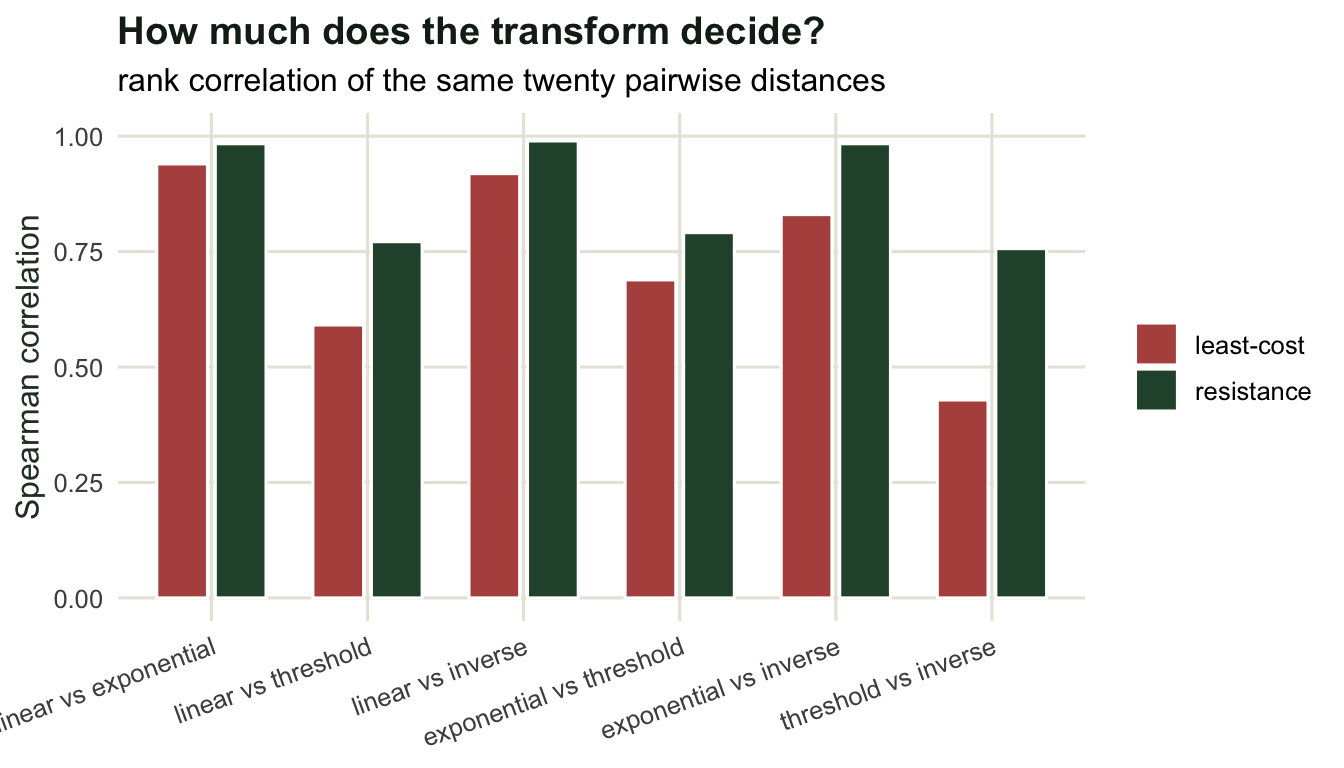
Check 4: change the grain

The last check is the one from the fragmentation tutorial, applied to distances. Aggregate the quality surface by two and recompute.

aggregate2 <- function(m) {
  k <- floor(nrow(m) / 2)
  out <- matrix(0, k, k)
  for (i in seq_len(k)) {
    for (j in seq_len(k)) {
      out[i, j] <- mean(m[(2 * i - 1):(2 * i), (2 * j - 1):(2 * j)])
    }
  }
  out
}

qual_c <- aggregate2(qual)
nc <- nrow(qual_c)
res_c <- 1 + 99 * (1 - qual_c)
tgt_c <- pmin(nc, c(ceiling(tgt_xy[1] / 2), ceiling(tgt_xy[2] / 2)))
src_c <- cbind(pmin(nc, ceiling(src_xy[, 1] / 2)),
               pmin(nc, ceiling(src_xy[, 2] / 2)))
snk_c <- matrix(FALSE, nc, nc)
snk_c[tgt_c[1], tgt_c[2]] <- TRUE
lcp_c <- cost_distance(res_c, snk_c)[src_c]
tgt_node_c <- (tgt_c[2] - 1) * nc + tgt_c[1]
src_node_c <- (src_c[, 2] - 1) * nc + src_c[, 1]
ok <- src_node_c != tgt_node_c
kit_c <- resistance_kit(res_c)
reff_c <- sapply(src_node_c[ok], function(s) r_eff_pair(kit_c, s, tgt_node_c))

cat("pairs usable at both grains:", sum(ok), "\n")

pairs usable at both grains: 20 

cat("fine against coarse, rank correlation: least-cost", sp(lcp[ok], lcp_c[ok]),
    " resistance", sp(r_eff[ok], reff_c), "\n")

fine against coarse, rank correlation: least-cost 0.9846  resistance 0.9846 

cat("median ratio, coarse over fine: least-cost",
    round(median(lcp_c[ok]) / median(lcp[ok]), 4),
    " resistance", round(median(reff_c) / median(r_eff[ok]), 4), "\n")

median ratio, coarse over fine: least-cost 0.5101  resistance 0.9623 

The rankings survive: both metrics correlate at 0.9846 between grains, so a study that only compares pairs of sites is fairly safe. The absolute values do not survive. Least-cost distance halves (median ratio 0.5101) because halving the number of cells halves the number of steps, and effective resistance shifts by less (0.9623) because it is a ratio of voltages rather than a sum along a route.

So cost-distance values are not comparable across studies with different cell sizes, and any connectivity threshold expressed in cost units is tied to the grain it was calibrated on.

The honest limit

The deepest problem is not in this tutorial and cannot be. Every check above validates the machinery against itself: the circuit against the walk, one transform against another, one grain against another. None of them validates the resistance surface against nature, because the simulations have no organisms in them.

That validation requires independent data on movement or gene flow, which is why landscape genetics exists, and it is where this cluster meets the population genetics one. The standard approach regresses a genetic distance on candidate resistance distances and picks the surface that fits best, and the two measurements above set the bar it has to clear: the candidate surfaces must be distinguishable from each other (they correlated at 0.66 to 0.92 here) and better than straight-line distance (which predicted the walk at 0.9202). A resistance surface that beats Euclidean distance by a small margin on one data set has not been validated; it has been fitted.

Where to go next

The genetic side of this argument is built in the population genetics cluster, and the tutorial on drift, migration and isolation by distance is the direct counterpart to this one: it derives what geographic distance alone does to differentiation, which is exactly the null model a landscape genetics study has to beat.

References

Zeller KA, McGarigal K, Whiteley AR 2012 Landscape Ecology 27(6):777-797 (10.1007/s10980-012-9737-0)

Spear SF, Balkenhol N, Fortin MJ, McRae BH, Scribner K 2010 Molecular Ecology 19(17):3576-3591 (10.1111/j.1365-294X.2010.04657.x)

Chandra AK, Raghavan P, Ruzzo WL, Smolensky R, Tiwari P 1996 Computational Complexity 6(4):312-340 (10.1007/BF01270385)

Wu J 2004 Landscape Ecology 19(2):125-138 (10.1023/B:LAND.0000021711.40105.1a)

Related tutorials

• Patch metrics and fragmentation
• Least-cost paths and resistance surfaces
• Circuit theory and effective resistance
• Drift, migration and isolation by distance