library(ggplot2)
library(patchwork)

te_paper  <- "#f5f4ee"
te_ink    <- "#16241d"
te_body   <- "#2c3a31"
te_forest <- "#275139"
te_rust   <- "#b5534e"
te_gold   <- "#c9b458"
te_line   <- "#dad9ca"

theme_datasheet <- function() {
  theme_minimal(base_size = 12) +
    theme(plot.background  = element_rect(fill = te_paper, colour = NA),
          panel.background = element_rect(fill = te_paper, colour = NA),
          panel.grid.major = element_line(colour = te_line, linewidth = 0.3),
          panel.grid.minor = element_blank(),
          text             = element_text(colour = te_body),
          plot.title       = element_text(colour = te_ink, face = "bold"),
          plot.subtitle    = element_text(colour = te_body),
          axis.text        = element_text(colour = te_body))
}Patches cut by the edge of the map
R
landscape ecology
patch metrics
edge correction
simulation
ecology tutorial
Mean patch size from a map window is biased low, and dropping border patches is worse. Measuring the Miles-Lantuejoul edge correction for habitat patches in R.
A study of woodland birds takes a national land-cover raster at 25 m resolution and cuts a square of 2.5 km around each survey point: 100 cells a side. Inside every square it computes the usual patch statistics (mean patch size, the area-weighted mean, the largest patch index) and relates them to the bird counts. The square has an edge, and the woodland does not stop at it. A wood that runs out of the square is recorded as a patch of whatever area lies inside, and the software has no way of knowing that the rest exists.
Whether that matters has a precise answer, and it is old. Stereologists counting particles in microscope sections met the same problem decades ago: a particle cut by the edge of the field of view is measured short, and the fix that looks careful, ignoring every particle that touches the edge, selects against large particles. Miles (1978) set out the problem for planar aggregates sampled by quadrats, where the choice of whether to count particles truncated by the boundary had led to biased estimates, and gave an unbiased “associated point” rule: a particle is counted when one point uniquely associated with it falls in the quadrat, and it is then measured whole. The correction used for most of this post is a different one. It keeps only the particles that lie wholly inside the frame and weights each by the inverse of its chance of doing so; it is usually called the Miles-Lantuejoul or minus-sampling correction, and Baddeley and Jensen (2005) set out both rules with the other edge corrections of stereology. Nothing here is new. This post demonstrates that result on raster habitat patches, measures how large the two naive biases are for a smoothed neutral landscape, and finds where the correction itself stops working.
The blog has handled edges before, but for points and trees, not for patches. Nearest-neighbour analysis and Clark-Evans uses the border, or reduced-sample, estimator: a point only counts at distance r if it lies at least r from the boundary. Angle-count sampling for basal area compares a torus, a buffer and ignoring the slopover for trees near a stand edge. The patch statistics themselves were built in patch metrics and fragmentation, whose labeller pads the grid with non-habitat, so the edge of the grid acts as a real boundary; that post varies the habitat amount, the arrangement and the grain, and computes every metric on one whole grid. Checking a connectivity analysis also changes the grain in its fourth check. Neither of the two patch posts changes the extent, which is the variable here.
A map with no edge to be the truth
The reference has to be a map with no edge at all, or the truth is cut too. The population map below is a torus: the smoothing and the patch labelling both wrap around, so a patch that leaves the right-hand side continues on the left. The generator is the one from the patch metrics post (uniform noise, repeated local averaging, a threshold at a quantile), with the averaging wrapped. The labeller is the same four-neighbour label propagation, with a switch for the wrap. For each patch the chunk also stores its extent: the smallest run of rows and of columns that covers it on the torus, and the first row and column of that run, which is used as the patch’s associated cell in the last estimator.
wrap_idx <- function(v, n) ((v - 1) %% n) + 1

smooth_torus <- function(n, passes) {
  z  <- matrix(runif(n * n), n, n)
  up <- wrap_idx(0:(n - 1), n)
  dn <- wrap_idx(2:(n + 1), n)
  for (p in seq_len(passes)) {
    z <- (4 * z + z[up, ] + z[dn, ] + z[, up] + z[, dn]) / 8
  }
  z
}

# label propagation, four-neighbour; torus = TRUE wraps the edges
label_patches <- function(hab, torus = FALSE) {
  n <- nrow(hab); m <- ncol(hab)
  lab <- matrix(0L, n, m)
  lab[hab] <- seq_len(sum(hab))
  up <- wrap_idx(0:(n - 1), n); dn <- wrap_idx(2:(n + 1), n)
  repeat {
    old <- lab
    if (torus) {
      best <- pmax(lab, lab[up, ], lab[dn, ], lab[, up], lab[, dn])
    } else {
      best <- pmax(lab, rbind(0L, lab[-n, ]), rbind(lab[-1, ], 0L),
                   cbind(0L, lab[, -m]), cbind(lab[, -1], 0L))
    }
    lab[hab] <- best[hab]
    if (identical(lab, old)) break
  }
  lab
}

# smallest run of rows (or columns) that covers a patch on the torus
circ_span <- function(v, n) {
  u <- sort(unique(v))
  if (length(u) == n) return(n)
  n - max(diff(c(u, u[1] + n))) + 1
}

# first row (or column) of that run: the patch's associated cell
circ_start <- function(v, n) {
  u <- sort(unique(v))
  if (length(u) == n) return(1)
  u[(which.max(diff(c(u, u[1] + n))) %% length(u)) + 1]
}

torus_patches <- function(hab) {
  n <- nrow(hab)
  lab <- label_patches(hab, torus = TRUE)
  idx <- which(hab)
  f <- match(lab[idx], unique(lab[idx]))
  data.frame(area = tabulate(f),
             h = as.vector(tapply((idx - 1) %% n + 1, f, circ_span, n = n)),
             w = as.vector(tapply((idx - 1) %/% n + 1, f, circ_span, n = n)),
             r1 = as.vector(tapply((idx - 1) %% n + 1, f, circ_start, n = n)),
             c1 = as.vector(tapply((idx - 1) %/% n + 1, f, circ_start, n = n)))
}

n_map    <- 400     # cells per side of the population map
passes   <- 8       # smoothing passes
hab_frac <- 0.30    # habitat share

set.seed(2026)
z_map   <- smooth_torus(n_map, passes)
hab_map <- z_map >= quantile(z_map, 1 - hab_frac)
pop     <- torus_patches(hab_map)

pop_n     <- nrow(pop)
pop_mean  <- mean(pop$area)
pop_am    <- sum(pop$area^2) / sum(pop$area)
pop_max   <- max(pop$area)
pop_ext   <- pmax(pop$h, pop$w)
ext_max   <- max(pop_ext)
ext_q90   <- unname(quantile(pop_ext, 0.90))
pop_lpi   <- 100 * pop_max / n_map^2
wraps     <- sum(pop$h >= n_map | pop$w >= n_map)
The map has 400 cells a side, 30 per cent habitat and 1274 patches. Their mean area is 37.68 cells and the area-weighted mean is 160.6 cells, because a few large patches hold much of the habitat: the largest has 666 cells and spans 76 cells in its longer direction, while nine patches in ten span 18 cells or fewer. No patch wraps all the way round the torus (the chunk counts 0), so every patch has a finite extent. These are the population values every estimator below is compared with.
Three ways to average what a window shows
A window is a square of W cells placed at random on the torus and read as if it were a map of its own: the plane labeller, with no wrap, runs on the cells inside. Each patch in the window gets its area, the height and width of its bounding box, and a flag for whether any of its cells lies in the outer row or column. Three estimators of mean patch size follow. The first averages every patch in the window, cut or not. The second drops the patches that touch the border. The third keeps only the interior patches and weights each one.
The weight comes from counting placements. A patch whose bounding box is h rows by w columns lies inside a W by W window without touching the border only if its box sits within the inner W - 2 rows and columns, which leaves W - h - 1 row offsets and W - w - 1 column offsets. With the window placed uniformly over the torus, the chance of seeing that patch whole and untouched is therefore (W - h - 1)(W - w - 1) divided by the number of positions, and an interior patch that is seen is always the whole population patch, because any continuation would have to cross the border. Weighting each interior patch by one over the placement count is a Horvitz and Thompson (1952) estimator of the number of patches and, with the area in the numerator, of their total area. The ratio of the two estimates the mean.
window_patches <- function(hw) {
  W <- nrow(hw)
  lb <- label_patches(hw)
  ii <- which(hw)
  f <- match(lb[ii], unique(lb[ii]))
  rw <- (ii - 1) %% W + 1
  cw <- (ii - 1) %/% W + 1
  rmin <- tapply(rw, f, min); rmax <- tapply(rw, f, max)
  cmin <- tapply(cw, f, min); cmax <- tapply(cw, f, max)
  data.frame(area  = tabulate(f),
             h     = as.vector(rmax - rmin + 1),
             w     = as.vector(cmax - cmin + 1),
             touch = as.vector(rmin == 1 | cmin == 1 | rmax == W | cmax == W))
}

# Miles-Lantuejoul weight: one over the number of interior placements
ml_weight <- function(pw, W) {
  ifelse(pw$touch, 0, 1 / ((W - pw$h - 1) * (W - pw$w - 1)))
}

w_show  <- 50   # window side used for the examples
n_small <- 70   # side of the small torus for the exhaustive check
w_small <- 24   # window side for the exhaustive check
n_pos_small <- n_small^2

cut_window <- function(hab, r0, c0, W) {
  n <- nrow(hab)
  hab[wrap_idx(r0:(r0 + W - 1), n), wrap_idx(c0:(c0 + W - 1), n), drop = FALSE]
}set.seed(31)
r_demo <- sample.int(n_map - w_show, 1); c_demo <- sample.int(n_map - w_show, 1)
map_df <- data.frame(x = rep(seq_len(n_map), each = n_map),
y = rep(seq_len(n_map), times = n_map),
habitat = as.vector(hab_map))
p_map <- ggplot(map_df[map_df$habitat, ], aes(x, y)) +
geom_raster(fill = te_forest) +
annotate("rect", xmin = c_demo - 0.5, xmax = c_demo + w_show - 0.5,
ymin = r_demo - 0.5, ymax = r_demo + w_show - 0.5,
fill = NA, colour = te_rust, linewidth = 0.8) +
coord_equal(expand = FALSE, xlim = c(0.5, n_map + 0.5), ylim = c(0.5, n_map + 0.5)) +
labs(x = NULL, y = NULL, title = "Population map") +
theme_datasheet() +
theme(axis.text = element_blank(), panel.grid.major = element_blank())
hw_demo <- hab_map[r_demo:(r_demo + w_show - 1), c_demo:(c_demo + w_show - 1)]
lb_demo <- label_patches(hw_demo)
pw_demo <- window_patches(hw_demo)
ids_demo <- unique(lb_demo[hw_demo])
touch_demo <- pw_demo$touch[match(lb_demo, ids_demo)]
win_df <- data.frame(x = rep(seq_len(w_show), each = w_show),
y = rep(seq_len(w_show), times = w_show),
habitat = as.vector(hw_demo))
win_df$status <- ifelse(win_df$habitat, ifelse(touch_demo, "touches the border", "interior"), NA)
p_win <- ggplot(win_df[win_df$habitat, ], aes(x, y, fill = status)) +
geom_raster() +
coord_equal(expand = FALSE, xlim = c(0.5, w_show + 0.5), ylim = c(0.5, w_show + 0.5)) +
scale_fill_manual(values = c(interior = te_forest, `touches the border` = te_rust)) +
labs(x = NULL, y = NULL, fill = NULL, title = "One window") +
theme_datasheet() +
theme(axis.text = element_blank(), panel.grid.major = element_blank(),
panel.border = element_rect(fill = NA, colour = te_rust, linewidth = 0.8),
legend.position = "bottom")
n_demo <- nrow(pw_demo); n_demo_touch <- sum(pw_demo$touch)
demo_in_max <- max(pw_demo$area[!pw_demo$touch])
demo_big_n <- sum(pw_demo$area > demo_in_max)
demo_big_max <- max(pw_demo$area)
p_map + p_win + plot_annotation(theme = theme_datasheet())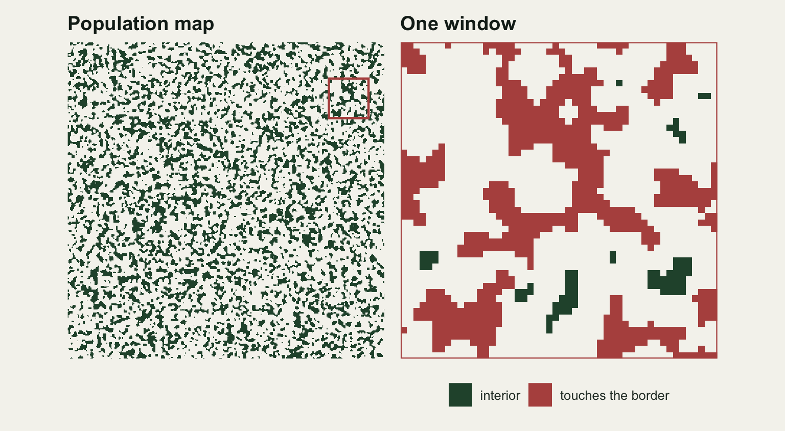
The window in the figure is one random draw at 50 cells, not a chosen one. Of its 20 patches, 12 touch the border. The largest interior patch has 28 cells; 6 patches are larger than that, up to 376 cells, and every one of them touches the border.
The placement argument is the whole claim of the correction, so it is worth checking by brute force rather than taking it on trust. On a small torus of 70 cells a side, a window of 24 cells is placed at every one of the 4900 possible positions, the window is labelled afresh each time, and the weights are summed. If the count (W - h - 1)(W - w - 1) is exact for four-neighbour raster patches, the sum over all positions equals the number of population patches that can fit, and the weighted areas sum to their total area, with no sampling error at all.
set.seed(78)
z_small   <- smooth_torus(n_small, passes)
hab_small <- z_small >= quantile(z_small, 1 - hab_frac)
pop_small <- torus_patches(hab_small)

sum_w <- 0; sum_wa <- 0
for (r0 in seq_len(n_small)) {
  for (c0 in seq_len(n_small)) {
    hw <- cut_window(hab_small, r0, c0, w_small)
    if (!any(hw)) next
    pw <- window_patches(hw)
    wt <- ml_weight(pw, w_small)
    sum_w  <- sum_w + sum(wt)
    sum_wa <- sum_wa + sum(wt * pw$area)
  }
}
fits_small   <- pop_small$h <= w_small - 2 & pop_small$w <= w_small - 2
n_fit_small  <- sum(fits_small)
a_fit_small  <- sum(pop_small$area[fits_small])
gap_count    <- abs(sum_w - n_fit_small)
gap_area     <- abs(sum_wa - a_fit_small)
The weights sum to 48.000000 over all positions, against 48 patches on the small torus whose extent is at most W - 2 in both directions; the weighted areas sum to 1028.000000 against their total of 1028 cells. The differences, 5.0e-14 and 1.1e-12, are rounding. The small torus has 49 patches in all, and the one that is missing from the sum is too large to fit: it gets no weight because it can never be seen whole. That is the identity, and it also names the failure. The weighting is exact for the patches that fit in the window and silent about the ones that do not.
Cut patches pull the mean down; dropping them pulls harder
The sweep places random windows of eight sizes on the population map. The number of windows was fixed before running at 1000 for the four smaller sizes, 500 at 70 cells and 200 above that, because small windows are cheap to label and the weighted estimator is noisy in them. Each estimator is pooled over the windows of one size as a ratio (the sum of the areas over the sum of the counts, weighted where the estimator is weighted), and its Monte Carlo standard error comes from the delta method for a ratio. For the weighted estimator the chunk also records the mean area of the population patches that can fit at that size, which is what the identity says it estimates.
w_set  <- c(20, 25, 35, 50, 70, 100, 140, 200)
n_win  <- ifelse(w_set <= 50, 1000, ifelse(w_set <= 70, 500, 200))

set.seed(908)
win_rows <- vector("list", sum(n_win))
piece_rows <- list()
j <- 0
for (i in seq_along(w_set)) {
  W <- w_set[i]
  for (k in seq_len(n_win[i])) {
    j <- j + 1
    r0 <- sample.int(n_map, 1); c0 <- sample.int(n_map, 1)
    hw <- cut_window(hab_map, r0, c0, W)
    if (!any(hw)) {
      win_rows[[j]] <- c(W, rep(0, 10), r0, c0)
      next
    }
    pw <- window_patches(hw)
    wt <- ml_weight(pw, W)
    a  <- pw$area
    inn <- !pw$touch
    win_rows[[j]] <- c(W, length(a), sum(a), sum(a^2), sum(inn), sum(a[inn]),
                       sum(a[inn]^2), sum(wt), sum(wt * a), sum(wt * a^2),
                       max(a), r0, c0)
    if (W == w_show) piece_rows[[length(piece_rows) + 1]] <- pw[, c("area", "touch")]
  }
}
win <- as.data.frame(do.call(rbind, win_rows))
names(win) <- c("W", "n_all", "a_all", "a2_all", "n_in", "a_in", "a2_in",
                "s_w", "s_wa", "s_wa2", "a_max", "r0", "c0")
pieces <- do.call(rbind, piece_rows)

# pooled ratio over windows, with a delta-method Monte Carlo standard error
ratio_se <- function(y, x) {
  r <- sum(y) / sum(x)
  k <- length(x)
  c(est = r, se = sqrt(sum((y - r * x)^2) * k / (k - 1)) / sum(x))
}

summ <- do.call(rbind, lapply(w_set, function(W) {
  d <- win[win$W == W, ]
  fits <- pop$h <= W - 2 & pop$w <= W - 2
  tr <- ratio_se(d$a_all, d$n_all)
  ex <- ratio_se(d$a_in, d$n_in)
  ml <- ratio_se(d$s_wa, d$s_w)
  data.frame(W = W, windows = nrow(d),
             trunc = tr[["est"]], trunc_se = tr[["se"]],
             excl = ex[["est"]], excl_se = ex[["se"]],
             ml = ml[["est"]], ml_se = ml[["se"]],
             fit_mean = mean(pop$area[fits]), fit_share = mean(fits),
             touch = 1 - sum(d$n_in) / sum(d$n_all))
}))
rel <- function(col) summ[[col]] / pop_mean
row_of <- function(W) which(summ$W == W)
excl_below <- all(summ$excl < summ$trunc)
z_ml       <- (summ$ml / pop_mean - 1) / (summ$ml_se / pop_mean)
z_fit      <- (summ$ml - summ$fit_mean) / summ$ml_se
w_fit_all  <- min(summ$W[summ$fit_share == 1])
z_big_max  <- max(abs(z_ml[summ$W >= 70]))
At the smallest window of 20 cells, keeping the cut patches gives 0.551 of the population mean, and dropping the border-touching ones gives 0.269. At 50 cells the two are 0.766 and 0.547, and even at 200 cells, half the side of the population map, they are 0.929 and 0.876. Dropping the touching patches is below keeping them at every window size (true for all eight). The share of patches in a window that touch the border falls from 0.73 to 0.14 over the same range.
The weighted ratio is a different story at the two ends. From 70 cells upwards it sits at 0.986, 1.022, 1.011 and 0.999 of the population mean, at most 1.0 Monte Carlo standard errors from one. Below that it is low wherever its standard error allows a verdict. At 50 cells it gives 0.890 with a standard error of 0.031, which is 3.5 standard errors short of the truth but only 0.8 from the mean of the patches that can fit (0.916). At 20 cells it gives 0.508 against a fitting mean of 0.533, and there it is no better than simply keeping the cut patches (0.551, a gap smaller than its standard error of 0.049), although 90 per cent of the population patches can fit: the patches that cannot are the large ones, and they carry the mean. Every population patch can fit only once the window is 78 cells, two more than the largest extent (the grey vertical line); the first size in the sweep above that is 100 cells.
At 35 cells the weighted estimate is 0.968, but its standard error is 0.175 even from 1000 windows, so that point says nothing either way. The weight of a patch whose box fills the inner square is one, while a single cell gets one over (W - 2) squared, so one window that happens to hold a large patch whole can outweigh hundreds of others. That heavy tail is the price of the correction, and it returns in the single-window section below.
bias_df <- rbind(
  data.frame(W = summ$W, est = rel("trunc"), se = summ$trunc_se / pop_mean,
             estimator = "all patches, cut ones included"),
  data.frame(W = summ$W, est = rel("excl"), se = summ$excl_se / pop_mean,
             estimator = "border-touching patches dropped"),
  data.frame(W = summ$W, est = rel("ml"), se = summ$ml_se / pop_mean,
             estimator = "interior patches, Miles-Lantuejoul weights"))
fit_df <- data.frame(W = summ$W, est = rel("fit_mean"))

ggplot(bias_df, aes(W, est, colour = estimator)) +
  geom_hline(yintercept = 1, colour = te_ink, linetype = "dashed", linewidth = 0.4) +
  geom_vline(xintercept = ext_max + 2, colour = te_line, linewidth = 0.8) +
  geom_line(data = fit_df, aes(W, est), inherit.aes = FALSE,
            colour = te_body, linetype = "dotted", linewidth = 0.6) +
  geom_errorbar(aes(ymin = est - 2 * se, ymax = est + 2 * se), width = 0.03) +
  geom_line(linewidth = 0.7) +
  geom_point(size = 2) +
  scale_x_log10(breaks = w_set) +
  scale_colour_manual(values = c(`all patches, cut ones included` = te_gold,
                                 `border-touching patches dropped` = te_rust,
                                 `interior patches, Miles-Lantuejoul weights` = te_forest)) +
  labs(x = "window side (cells, log scale)",
       y = "estimate / population mean",
       colour = NULL,
       title = "Mean patch size seen through a window",
       subtitle = "error bars: two Monte Carlo standard errors; dotted: mean of patches that can fit") +
  theme_datasheet() +
  theme(legend.position = "bottom", legend.direction = "vertical")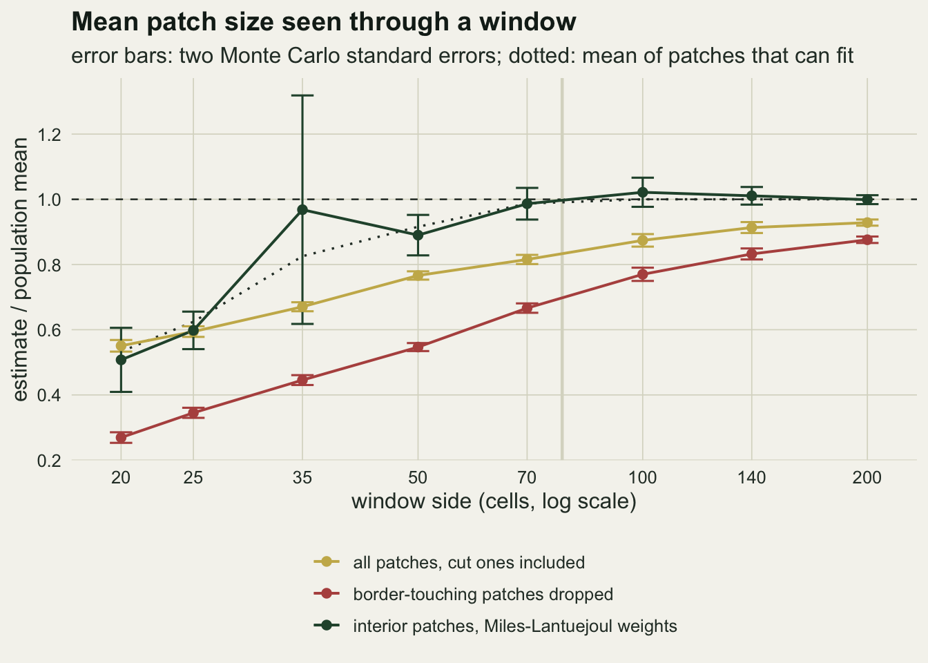
Two things might be expected: that dropping the touching patches fixes the bias, and that the weighted estimator fixes it once the window is a few patch diameters wide. The first is wrong at every size here. The second holds from 70 cells, which is about the extent of the largest patch rather than a few times the extent of a typical one, and below it the estimate is low wherever its standard error is small enough to tell, for the reason the identity gave.
Big patches are the ones that touch
Why dropping the touching patches is worse than keeping them is visible in the patches themselves. The chunk groups every patch seen in the 1000 windows of 50 cells by its visible area and records the share that touches the border.
size_breaks <- c(0, 1, 4, 16, 64, 256, Inf)
size_lab    <- c("1", "2-4", "5-16", "17-64", "65-256", "over 256")
pieces$size_class <- cut(pieces$area, size_breaks, labels = size_lab)
touch_by_size <- aggregate(touch ~ size_class, data = pieces, FUN = mean)
count_by_size <- as.vector(table(pieces$size_class))
touch_by_size$pieces <- count_by_size
touch_small <- touch_by_size$touch[1]
touch_big   <- touch_by_size$touch[nrow(touch_by_size)]
area_touch_share <- sum(pieces$area[pieces$touch]) / sum(pieces$area)
count_touch_share <- mean(pieces$touch)
Even among single cells 0.31 touch the border, far more than the 0.08 share of the window’s cells that lie in the outer ring, because many of them are the tips of larger patches that only just reach into the window. Among the visible patches larger than 256 cells the share is 0.94. Across all sizes the touching patches are 0.44 of the patches but hold 0.60 of the habitat area inside the windows. Dropping them removes a minority of patches and the majority of the area, and what remains is a sample of small patches.
ggplot(touch_by_size, aes(size_class, touch)) +
  geom_col(fill = te_forest, width = 0.7) +
  geom_text(aes(label = sprintf("n = %d", pieces)), vjust = -0.5,
            colour = te_body, size = 3.4) +
  scale_y_continuous(limits = c(0, 1.08), breaks = seq(0, 1, 0.25)) +
  labs(x = "area of the patch inside the window (cells)",
       y = "share touching the border",
       title = "The larger the patch, the more likely it is cut",
       subtitle = sprintf("%d random windows of %d by %d cells", n_win[w_set == w_show], w_show, w_show)) +
  theme_datasheet()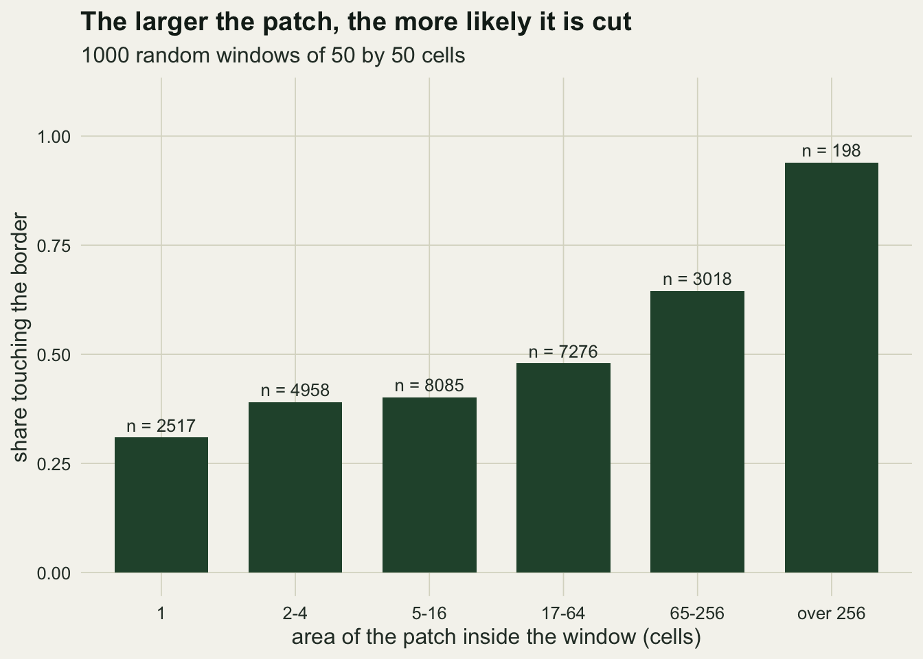
A cut patch is still counted in the first estimator, only short. Removing it removes a large patch altogether, and the probability of removal rises with the size, which is a selection bias on top of the truncation. The weighted estimator also drops the touching patches, but it then gives the surviving large patches the weight they need to stand for the ones that were dropped.
The weights are a pooling tool, not a single-map fix
Pooling a thousand windows is what a stereologist does with a thousand fields of view. A landscape study often has one map per site and wants one number per map. The chunk below computes the uncorrected and the weighted estimators inside every single window and asks how far each one is from the population mean, as a relative root mean squared error. Windows with no interior patch give the weighted ratio nothing to divide and are left out of its error.
per_win <- do.call(rbind, lapply(w_set, function(W) {
  d <- win[win$W == W & win$n_all > 0, ]
  tr <- d$a_all / d$n_all / pop_mean
  ml <- d$s_wa / d$s_w / pop_mean
  ok <- is.finite(ml)
  data.frame(W = W,
             rmse_trunc = sqrt(mean((tr - 1)^2)),
             rmse_ml    = sqrt(mean((ml[ok] - 1)^2)),
             bias_ml_pw = mean(ml[ok]) - 1,
             no_interior = mean(!ok))
}))
pw_row <- function(W) which(per_win$W == W)
ml_worse_below <- all(per_win$rmse_ml[per_win$W < 200] > per_win$rmse_trunc[per_win$W < 200])
# associated-cell rule: count a population patch when its associated cell
# lies in the window, and use its whole area (needs the map beyond the window)
assoc <- do.call(rbind, lapply(w_set, function(W) {
  d <- win[win$W == W, ]
  in_r <- outer(pop$r1, d$r0, function(a, b) (a - b) %% n_map < W)
  in_c <- outer(pop$c1, d$c0, function(a, b) (a - b) %% n_map < W)
  hit <- in_r & in_c
  cnt <- colSums(hit)
  tot <- colSums(hit * pop$area)
  pooled <- ratio_se(tot, cnt)
  ok <- cnt > 0
  one <- tot[ok] / cnt[ok] / pop_mean
  data.frame(W = W, pooled = pooled[["est"]] / pop_mean, pooled_se = pooled[["se"]] / pop_mean,
             rmse_ap = sqrt(mean((one - 1)^2)), bias_ap_pw = mean(one) - 1,
             no_assoc = mean(!ok))
}))
z_ap_max    <- max(abs(assoc$pooled - 1) / assoc$pooled_se)
ap_above_trunc <- all(assoc$rmse_ap[assoc$W < 200] > per_win$rmse_trunc[per_win$W < 200])
ap_below_ml_from <- min(assoc$W[assoc$rmse_ap < per_win$rmse_ml])
ap_below_ml_rest <- all(assoc$rmse_ap[assoc$W >= ap_below_ml_from] <
                        per_win$rmse_ml[per_win$W >= ap_below_ml_from])
pool_rel_20 <- rel("ml")[row_of(20)] - 1
pool_rel_50 <- rel("ml")[row_of(50)] - 1
bias_pw_big <- max(abs(per_win$bias_ml_pw[per_win$W >= 70]))
The single-window weighted ratio has the larger error at every size below 200 cells (all seven): 0.67 against 0.30 at 50 cells, and 0.33 against 0.19 at 100. The two meet at 200 cells (0.100 and 0.097). In small windows the single-window ratio is also more biased than the pooled one: its mean relative error is -0.68 at 20 cells (pooled -0.49) and -0.15 at 50 (pooled -0.11), because most windows do not contain a large interior patch and the few that do are averaged in with equal standing. From 70 cells up it is within 0.042 of zero, so above that size its larger error is variance rather than bias. At 20 cells, 0.229 of the windows had no interior patch at all.
When the map beyond the window exists, the edge can be avoided instead of corrected, with the associated-point rule of Miles (1978). The chunk gives every population patch one associated cell (the first row and column of its extent), counts the patch in a window when that cell falls inside, and uses the patch’s whole area, read from the full map. For the same windows, the pooled ratio is within 1.1 standard errors of the population mean at every size, from 0.968 at 20 cells to 0.997 at 200, so it shows no large-patch failure. One window at a time (leaving out the windows that own no associated cell, 0.033 of them at 20 cells), it does not beat the uncorrected mean below the largest size: its relative RMSE is 1.13 at 20 cells and 1.03 at 25, above even the weighted ratio (0.76 and 0.70), then 0.43 at 50 and 0.08 at 200. It is below the weighted ratio from 35 cells up (at every such size) and above the uncorrected mean at every size below 200 (all seven); at 200 cells it is the lowest of the three. A small window that happens to own the associated cell of a large patch reports its full area, which keeps the pooled ratio on target and the single-window variance large; the single-window mean relative error is 0.06 at 20 cells and 0.06 at 50.
rmse_df <- rbind(
  data.frame(W = per_win$W, rmse = per_win$rmse_trunc, estimator = "all patches, cut ones included"),
  data.frame(W = per_win$W, rmse = per_win$rmse_ml, estimator = "Miles-Lantuejoul, one window"),
  data.frame(W = assoc$W, rmse = assoc$rmse_ap, estimator = "associated cell, whole patch"))
ggplot(rmse_df, aes(W, rmse, colour = estimator)) +
  geom_line(linewidth = 0.7) +
  geom_point(size = 2) +
  scale_x_log10(breaks = w_set) +
  scale_colour_manual(values = c(`all patches, cut ones included` = te_gold,
                                 `Miles-Lantuejoul, one window` = te_forest,
                                 `associated cell, whole patch` = te_rust)) +
  labs(x = "window side (cells, log scale)", y = "relative RMSE, one window",
       colour = NULL, title = "One map, one estimate") +
  theme_datasheet() +
  theme(legend.position = "bottom", legend.direction = "vertical")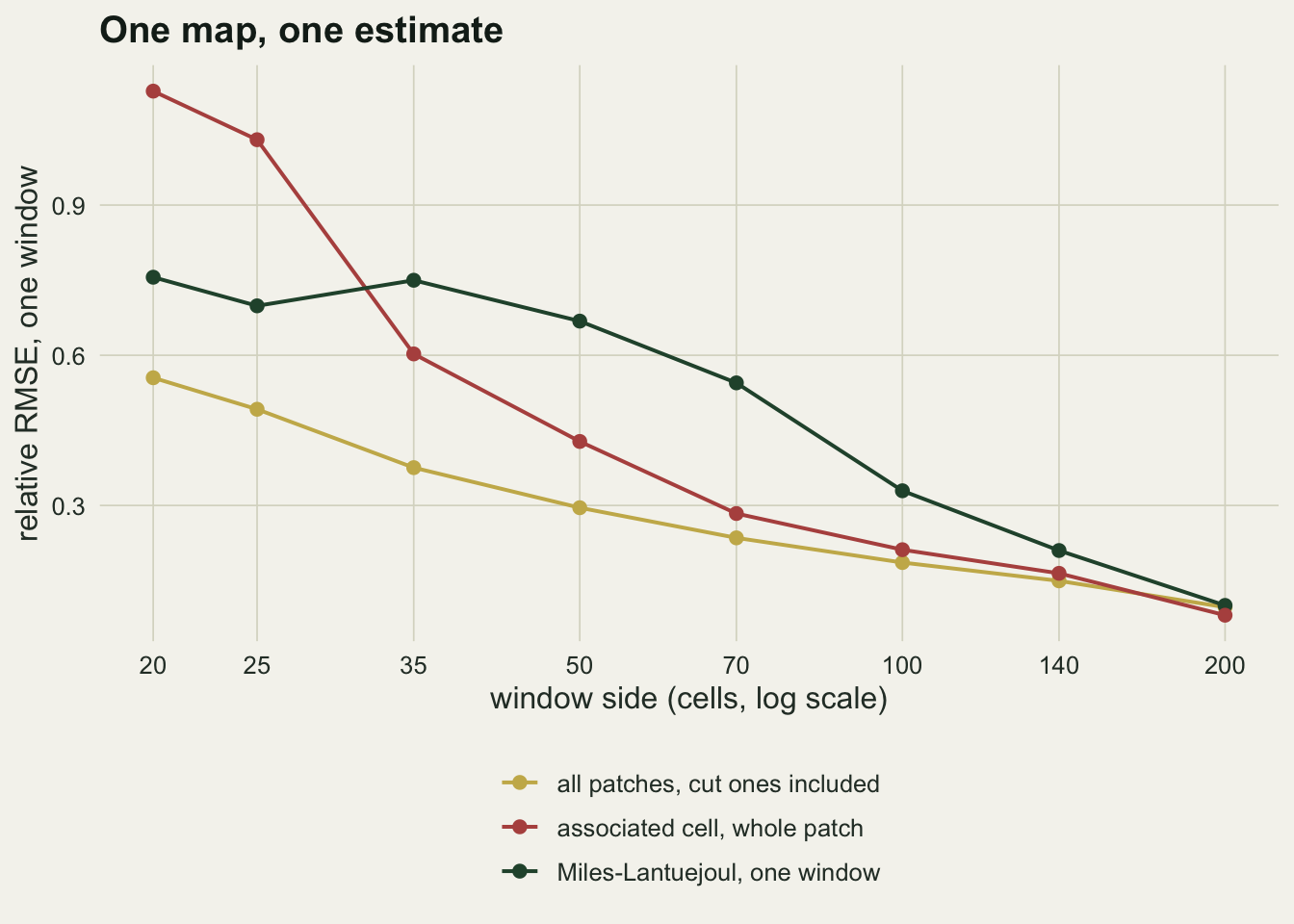
The small error belongs to the sum over windows, not to any one of them. For one map the weights trade a known downward bias for a large variance, and in this landscape that trade lost at every smaller window and only drew level when the window side was 2.6 times the extent of the largest patch.
Area-weighted mean and the largest patch index
FRAGSTATS also reports the area-weighted mean patch size (the sum of squared areas over the total area) and the largest patch index (the largest patch as a percentage of the landscape), and many studies use those instead of the plain mean. The first has a population value on the torus and the same three estimators apply to it: squared areas over areas, with the same weights for the corrected one. The second has no such value, because it is defined relative to the extent of the map, and the chunk only records how it moves.
frag <- do.call(rbind, lapply(w_set, function(W) {
  d <- win[win$W == W, ]
  tr <- ratio_se(d$a2_all, d$a_all)
  ex <- ratio_se(d$a2_in, d$a_in)
  ml <- ratio_se(d$s_wa2, d$s_wa)
  data.frame(W = W, am_trunc = tr[["est"]] / pop_am, am_excl = ex[["est"]] / pop_am,
             am_ml = ml[["est"]] / pop_am, am_ml_se = ml[["se"]] / pop_am,
             lpi = mean(100 * d$a_max / W^2))
}))
fr_row <- function(W) which(frag$W == W)
lpi_ratio_small <- frag$lpi[1] / pop_lpi
lpi_ratio_big   <- frag$lpi[nrow(frag)] / pop_lpi
am_excl_below   <- all(frag$am_excl < frag$am_trunc)
The area-weighted mean is hit harder by the edge than the plain mean, since it is carried by the large patches that are most often cut. Keeping cut patches gives 0.378 of the population value at 20 cells and 0.819 at 100; dropping them gives 0.156 and 0.749, below the first at every size (all eight). The weighted ratio reaches 1.033 at 100 cells (standard error 0.051) and 1.005 at 200. In the two smallest windows, though, it is below the uncorrected estimator: 0.285 against 0.378 at 20 cells and 0.337 against 0.438 at 25. A cut large patch still adds its square to the uncorrected sum, while the weighted sum has nothing at all for a patch that cannot fit. So the ranking of the plain mean carries over only in part: dropping touching patches is the worst choice throughout, but for the area-weighted mean the correction is worse than doing nothing in the two smallest windows, above it from 35 cells, and above it by more than its standard error from 50 cells, where the largest patches still do not fit (0.787 against 0.672 at 50 cells, standard error 0.065).
The largest patch index moves the other way. The whole map has an index of 0.42 per cent; windows of 20 cells average 17.0 per cent, 41 times as much, and windows of 200 cells still average 1.27 per cent, 3.0 times the whole-map value. The index divides by the area of the map, so a smaller map gives a larger index for the same woodland. There is no bias to correct because there is no extent-free quantity behind it; two index values are comparable only at the same extent.
am_df <- rbind(
  data.frame(W = frag$W, est = frag$am_trunc, estimator = "cut included"),
  data.frame(W = frag$W, est = frag$am_excl, estimator = "touching dropped"),
  data.frame(W = frag$W, est = frag$am_ml, estimator = "Miles-Lantuejoul"))
p_am <- ggplot(am_df, aes(W, est, colour = estimator)) +
  geom_hline(yintercept = 1, colour = te_ink, linetype = "dashed", linewidth = 0.4) +
  geom_line(linewidth = 0.7) +
  geom_point(size = 1.8) +
  scale_x_log10(breaks = c(20, 50, 100, 200)) +
  scale_colour_manual(values = c(`cut included` = te_gold, `touching dropped` = te_rust,
                                 `Miles-Lantuejoul` = te_forest)) +
  labs(x = "window side (cells)", y = "estimate / population value",
       colour = NULL, title = "Area-weighted mean") +
  theme_datasheet() +
  theme(legend.position = "bottom", legend.direction = "vertical")
p_lpi <- ggplot(frag, aes(W, lpi)) +
  geom_hline(yintercept = pop_lpi, colour = te_ink, linetype = "dashed", linewidth = 0.4) +
  geom_line(colour = te_forest, linewidth = 0.7) +
  geom_point(colour = te_forest, size = 1.8) +
  scale_x_log10(breaks = c(20, 50, 100, 200)) +
  scale_y_log10(breaks = c(0.3, 1, 3, 10)) +
  annotate("text", x = 200, y = pop_lpi * 1.25, label = "whole map", hjust = 1,
           colour = te_body, size = 3.4) +
  labs(x = "window side (cells)", y = "largest patch index (per cent, log)",
       title = "Largest patch index") +
  theme_datasheet()
p_am + p_lpi + plot_annotation(theme = theme_datasheet())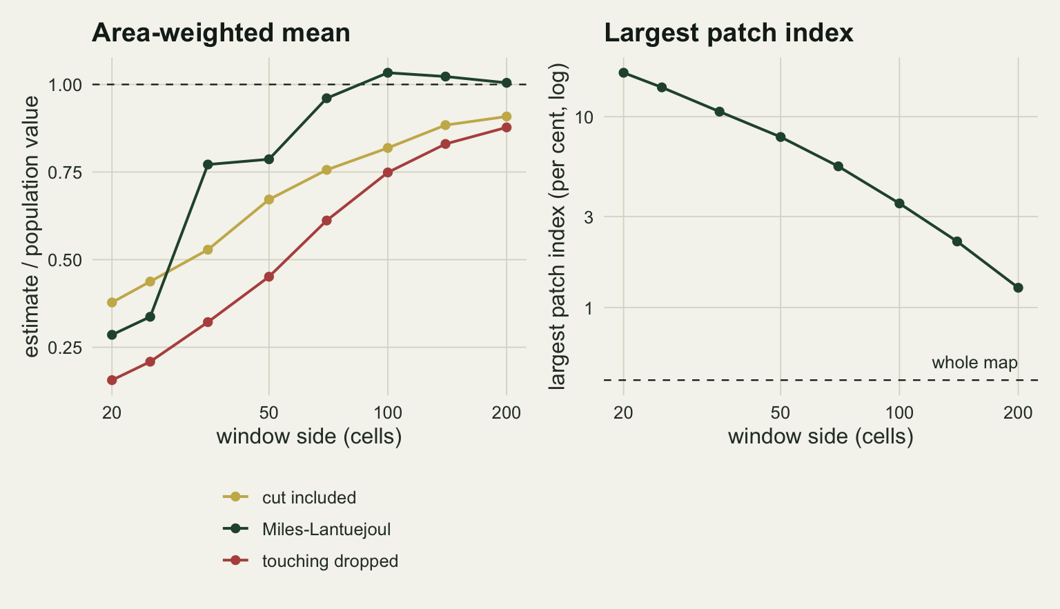
What to report
Li and Wu (2004) count the scale of the analysis among the conditions a landscape index cannot be read without, and scale has two parts: grain and extent. State the extent next to every patch statistic, in cells and in metres, together with the largest patch extent visible in the analysis squares; the ratio of the two is the number that tells a reader whether the statistics are cut. Do not drop the patches that touch the border to make the mean look cleaner: in this sweep that choice was the most biased of the three for both the plain and the area-weighted mean.
If many windows of the same size are pooled into one estimate, weight the interior patches by one over (W - h - 1)(W - w - 1) and pool as a ratio, and report the number of windows and a standard error that allows for a heavy tail. When the map beyond the square exists, as with a national raster, label the patches on the larger map, keep each patch whose associated cell lies in the square and use its full area: in this sweep the pooled rule stayed within 1.1 standard errors of the population mean at every window size, including those where the weights failed. If each map is analysed on its own, the uncorrected mean had a smaller error than either correction at every size below 200 cells, and it should be described as a mean of patches as seen through a square of that size, which in this landscape was below the population mean at every size tested. Largest patch index values from squares of different sizes should not be compared at all.
Honest limits
Everything above comes from one population map, one habitat share and one amount of smoothing. The standard errors describe windows drawn from that map, not landscapes drawn from a process; a second map with a different largest patch would move the size at which the correction starts to work, because that size followed the largest extent and not the typical one.
The smoothed-noise patches are compact. Hedgerows, riparian strips and forest along a valley have bounding boxes far larger than their areas, so they stop fitting in a window at a much smaller area, and every failure described here arrives at larger window sizes for them. The four-neighbour rule was used throughout. FRAGSTATS and landscapemetrics default to eight neighbours, under which diagonal contacts join patches and extents grow. The placement argument carries over, since a diagonal step out of a cell clear of the outer ring still lands inside the window, but the eight-neighbour rule was not run here, and the window sizes at which each estimator recovers under it were not measured. The associated-cell rule was checked on a torus, where every patch can be measured whole; on a real national raster the patches that run off that raster’s own edge bring the problem back one level up, and near a coast or border they are not rare.
Windows were placed uniformly over the map. Survey squares centred on nest sites, on woodland, or kept away from roads are not uniform, and then the chance of seeing a patch whole is not the placement count divided by the number of positions: the weights stay proportional to it only if the placement is unrelated to where patches lie. The window positions were drawn independently, so the standard errors are valid for placements on this map; at 200 cells each window covers a quarter of the torus, and the 200 windows describe that one map thoroughly and say nothing about another.
The delta-method standard error of the weighted ratio is itself unreliable when one window dominates the sum, as it did at 35 cells. Whether the corrected mean has recovered at that size cannot be settled from these windows, and a bootstrap over windows would not fix a tail that the sample has barely reached.
References
Miles RE 1978 Journal of Microscopy 113(3):257-267 (10.1111/j.1365-2818.1978.tb00104.x)
Baddeley A, Jensen EBV 2005 Stereology for Statisticians (ISBN 978-1-58488-405-7)
Horvitz DG, Thompson DJ 1952 Journal of the American Statistical Association 47(260):663-685 (10.1080/01621459.1952.10483446)
Li H, Wu J 2004 Landscape Ecology 19(4):389-399 (10.1023/B:LAND.0000030441.15628.d6)