library(ggplot2)

te_paper  <- "#f5f4ee"
te_ink    <- "#16241d"
te_body   <- "#2c3a31"
te_forest <- "#275139"
te_rust   <- "#b5534e"
te_gold   <- "#c9b458"
te_line   <- "#dad9ca"

theme_datasheet <- function() {
  theme_minimal(base_size = 12) +
    theme(plot.background  = element_rect(fill = te_paper, colour = NA),
          panel.background = element_rect(fill = te_paper, colour = NA),
          panel.grid.major = element_line(colour = te_line, linewidth = 0.3),
          panel.grid.minor = element_blank(),
          text             = element_text(colour = te_body),
          plot.title       = element_text(colour = te_ink, face = "bold"),
          plot.subtitle    = element_text(colour = te_body),
          axis.text        = element_text(colour = te_body))
}Angle-count sampling for basal area
R
forest inventory
survey design
sampling
simulation
ecology tutorial
Bitterlich angle counts sample trees in proportion to basal area. In R: the closed-form precision trade-off, how clumping shrinks it, and borderline-tree bias.
A forest ecologist stands at a sample point in a mixed oak and hornbeam stand with a wedge prism held over the point. She turns a full circle and counts every stem whose displaced image does not break away from the trunk seen above the glass. The count times the basal area factor of the prism is the basal area of the stand at that point, in square metres per hectare, and she has not measured a single diameter. The same count gives nothing about how many stems there are per hectare, and a colleague walking a fixed circular plot a few paces away has the opposite problem: stem density falls out of his tally directly, and basal area needs every diameter.
The trick behind the prism is sampling with probability proportional to size, a method Grosenbaugh (1952) introduced to North American foresters a few years after Bitterlich devised the gauge. A tree is counted when the point lies within a circle around the tree whose radius grows with the tree’s diameter, so a tree’s chance of entering the sample is proportional to its basal area, and each counted tree stands for the same amount of basal area per hectare. Unequal inclusion probabilities that a designer sets on purpose are in unequal probability spatial sampling, which ends by noting that unequal probabilities pay off for a total only when the probabilities are close to proportional to the values being added up. Here the probability is set by the tree’s own diameter, and the same weighting that helps one per-hectare total hurts the other. The size bias is the one in measuring animal speed from camera traps, where fast animals are photographed more often and the harmonic mean of the recorded speeds recovers the true mean; stems per hectare from an angle count is the same correction, a sum of reciprocals of basal area.
The post builds a simulated stand, checks the limiting distance, the unbiasedness of both totals and the closed-form precision gap in a random stand (a smaller coefficient of variation for basal area and a larger one for stem density at equal field effort), then measures how clumping of the stems changes that gap, and works out from the tree list how a band of uncertain borderline trees biases the two totals.
A stand, a gauge and a limiting distance
A gauge with a basal area factor BAF, in square metres per hectare, counts a tree of diameter D when the point is closer to the tree than its limiting distance R = D / (2 sqrt(BAF)), with D in centimetres and R in metres. The gauge angle follows from the same geometry: half the diameter divided by the limiting distance is the sine of half the angle. Before any simulation the units deserve a numerical check, because a factor of one hundred in the wrong place still gives a plausible looking radius.
baf_set <- 4                                    # square metres per hectare
lim_dist <- function(dbh_cm, baf) dbh_cm / (2 * sqrt(baf))   # metres
dbh_chk <- 40
r_chk <- lim_dist(dbh_chk, baf_set)
g_chk <- pi * (dbh_chk / 200)^2                 # basal area of the tree, m2
zone_ha <- pi * r_chk^2 / 1e4                   # inclusion zone, hectares
per_ha_chk <- g_chk / zone_ha                   # should equal the BAF
angle_deg <- 2 * asin((dbh_chk / 200) / r_chk) * 180 / pi
baf_from_angle <- 1e4 * sin(angle_deg / 2 * pi / 180)^2
A tree of 40 cm is counted out to 10.00 m at a BAF of 4. Its basal area is 0.1257 square metres and its inclusion zone covers 0.03142 hectares, so the tree contributes 4.0000 square metres per hectare whenever it is counted, which is the BAF exactly. The gauge angle is 2.292 degrees, and ten thousand times the squared sine of half that angle gives back 4.0000. Every other diameter works the same way, since the inclusion zone and the basal area both grow with the square of the diameter.
The stand is a square of 200 m, four hectares, with 750 stems per hectare expected and a reverse-J diameter distribution: seven centimetres, the calliper threshold, plus an exponential with a mean of eleven centimetres. Clumping comes from a Thomas process, ten cluster centres per hectare with stems scattered around each centre by a normal displacement. Edges are removed by treating the square as a torus, so a point near the east side sees the trees near the west side; that makes the stand an infinite repetition of one tile and every point equally placed. A later section checks what a buffer instead of the torus does. The density, diameter distribution and BAF were fixed before any coefficient of variation was computed; the grid of cluster scatters was set after a pilot run.
side_m <- 200; area_ha <- side_m^2 / 1e4
n_ha <- 750; parents_ha <- 10; clump_sd_main <- 6
n_pts <- 2000
rev_j <- function(n) 7 + rexp(n, 1 / 11)
make_stand <- function(n_per_ha, clump_sd, dbh_fun) {
  n_tree <- rpois(1, n_per_ha * area_ha)
  if (is.na(clump_sd)) {
    xs <- runif(n_tree, 0, side_m); ys <- runif(n_tree, 0, side_m)
  } else {
    n_par <- rpois(1, parents_ha * area_ha)
    px <- runif(n_par, 0, side_m); py <- runif(n_par, 0, side_m)
    who <- sample.int(n_par, n_tree, replace = TRUE)
    xs <- (px[who] + rnorm(n_tree, 0, clump_sd)) %% side_m
    ys <- (py[who] + rnorm(n_tree, 0, clump_sd)) %% side_m
  }
  dbh <- dbh_fun(n_tree)
  data.frame(x = xs, y = ys, dbh = dbh, g = pi * (dbh / 200)^2)
}
stand_truth <- function(st) c(ba = sum(st$g) / area_ha, n = nrow(st) / area_ha)

# distances from a block of points to every tree, on the torus or the plane
dist_block <- function(px, py, st, torus) {
  dx <- abs(outer(px, st$x, "-")); dy <- abs(outer(py, st$y, "-"))
  if (torus) { dx <- pmin(dx, side_m - dx); dy <- pmin(dy, side_m - dy) }
  sqrt(dx^2 + dy^2)
}
# per point estimates of basal area and stems per hectare from both designs
tally <- function(st, pts, baf, r_fix, torus = TRUE, block = 200) {
  r_lim <- lim_dist(st$dbh, baf); a_fix <- pi * r_fix^2 / 1e4
  est <- matrix(0, nrow(pts), 4,
                dimnames = list(NULL, c("ba_angle", "n_angle", "ba_fixed", "n_fixed")))
  for (s in seq(1, nrow(pts), by = block)) {
    ii <- s:min(nrow(pts), s + block - 1)
    dd <- dist_block(pts$x[ii], pts$y[ii], st, torus)
    in_a <- sweep(dd, 2, r_lim, "<"); in_f <- dd < r_fix
    est[ii, 1] <- baf * rowSums(in_a)
    est[ii, 2] <- as.vector(in_a %*% (baf / st$g))
    est[ii, 3] <- as.vector(in_f %*% st$g) / a_fix
    est[ii, 4] <- rowSums(in_f) / a_fix
  }
  est
}
cv_of <- function(v) sd(v) / mean(v)
# fixed radius giving the same expected number of trees per point as the gauge
equal_radius <- function(truth, baf) sqrt((truth[["ba"]] / baf) * 1e4 / (pi * truth[["n"]]))
Equal effort needs a definition, and the one used here is the number of trees handled at a point. The expected angle count is the basal area per hectare divided by the BAF; the fixed plot radius is chosen so that its expected count, the stem density times the plot area, is the same number. On that definition both crews measure the same number of diameters per point on average. It is generous to the fixed plot where basal area is the target, because the angle count gets basal area without any diameter at all. For stem density it errs the other way: the angle count needs every counted diameter, the fixed plot only a threshold check.
set.seed(2608)
st_main <- make_stand(n_ha, clump_sd_main, rev_j)
tr_main <- stand_truth(st_main)
m_main <- tr_main[["ba"]] / baf_set
r_fix_main <- equal_radius(tr_main, baf_set)
pts_main <- data.frame(x = runif(n_pts, 0, side_m), y = runif(n_pts, 0, side_m))
est_main <- tally(st_main, pts_main, baf_set, r_fix_main)
max_r_main <- max(lim_dist(st_main$dbh, baf_set))
n_count_pt <- as.vector(est_main[, "ba_angle"] / baf_set)
i_show <- which(n_count_pt == round(m_main) & pts_main$x > 40 & pts_main$x < 160 &
                pts_main$y > 40 & pts_main$y < 160)[1]
The simulated stand has 3082 stems, 25.4 square metres of basal area per hectare and 770 stems per hectare. At a BAF of 4 the expected angle count is 6.34 trees per point, and a fixed plot of radius 5.12 m has the same expected count. The largest tree has a limiting distance of 24.9 m, far smaller than the 200 m tile.
p0 <- pts_main[i_show, ]
win <- 30
near <- st_main
near$dx <- (near$x - p0$x + side_m / 2) %% side_m - side_m / 2
near$dy <- (near$y - p0$y + side_m / 2) %% side_m - side_m / 2
near <- near[abs(near$dx) < win & abs(near$dy) < win, ]
near$dist <- sqrt(near$dx^2 + near$dy^2)
near$r_lim <- lim_dist(near$dbh, baf_set)
near$angle_in <- near$dist < near$r_lim
near$fixed_in <- near$dist < r_fix_main
near$status <- factor(ifelse(near$angle_in & near$fixed_in, "both",
                      ifelse(near$angle_in, "angle count only",
                      ifelse(near$fixed_in, "fixed plot only", "neither"))),
                      levels = c("angle count only", "fixed plot only", "both", "neither"))
circ <- function(cx, cy, r, id) {
  th <- seq(0, 2 * pi, length.out = 90)
  data.frame(x = cx + r * cos(th), y = cy + r * sin(th), id = id)
}
zones <- do.call(rbind, lapply(which(near$angle_in), function(i)
  circ(near$dx[i], near$dy[i], near$r_lim[i], i)))
plot_c <- circ(0, 0, r_fix_main, 0)
ggplot() +
  geom_path(data = zones, aes(x, y, group = id), colour = te_gold, linewidth = 0.4) +
  geom_path(data = plot_c, aes(x, y), colour = te_ink, linetype = "dashed", linewidth = 0.7) +
  geom_point(data = near, aes(dx, dy, size = dbh, colour = status), alpha = 0.9) +
  annotate("point", x = 0, y = 0, shape = 3, size = 4, stroke = 1.2, colour = te_ink) +
  scale_colour_manual(values = c("angle count only" = te_rust, "fixed plot only" = te_forest,
                                 "both" = te_ink, "neither" = "#9aa396"), name = NULL, drop = FALSE) +
  scale_size_continuous(range = c(0.6, 5), name = "DBH (cm)") +
  coord_equal(xlim = c(-win, win), ylim = c(-win, win)) +
  labs(x = "metres east of the point", y = "metres north of the point",
       title = "Who gets counted at one point",
       subtitle = "gold: inclusion zones of counted trees, dashed: fixed plot") +
  theme_datasheet()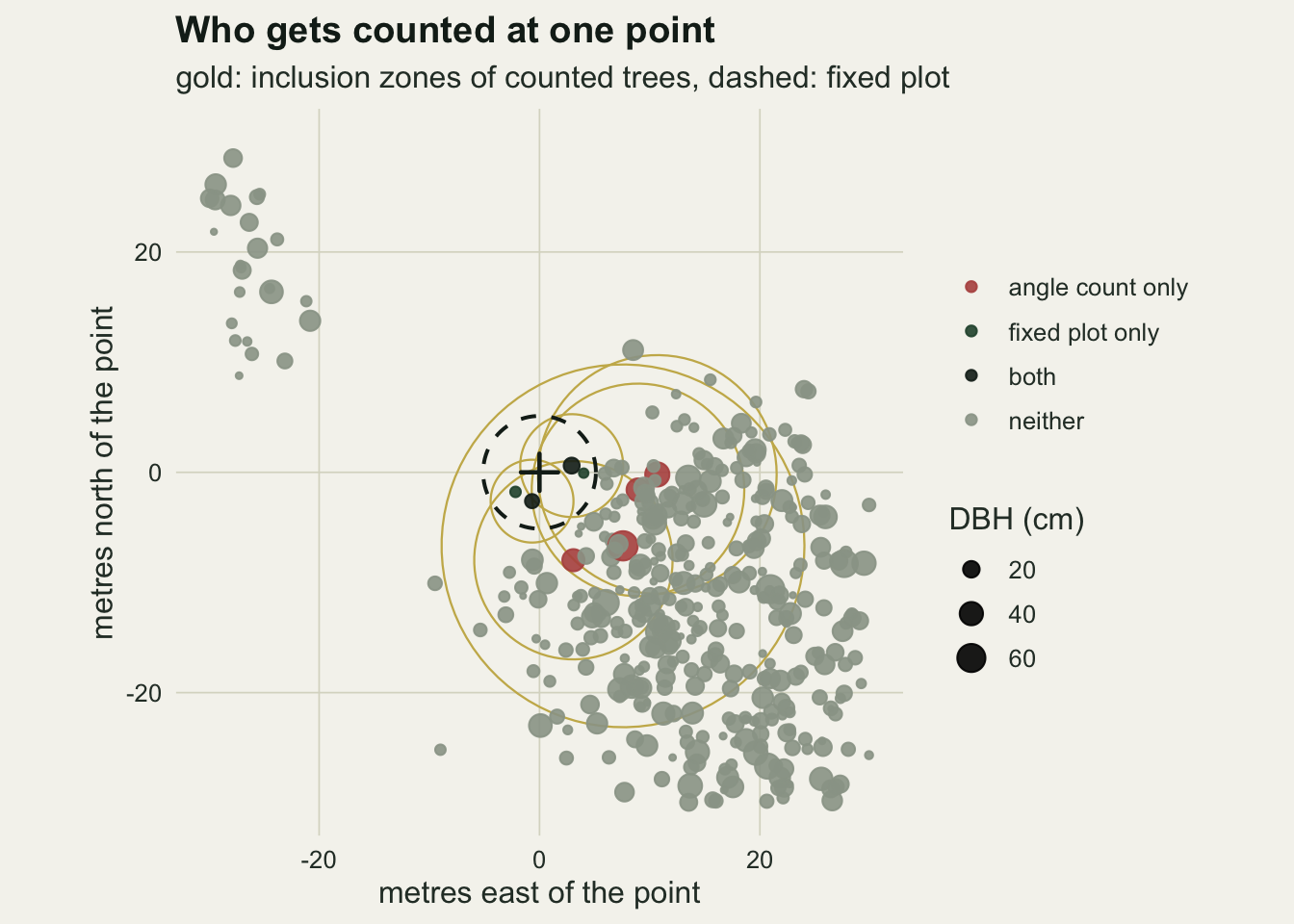
Both designs are unbiased; their spreads are not the same
On the torus a uniformly placed point falls in a tree’s inclusion zone with probability equal to the zone area divided by the stand area, so each counted tree weighted by the reciprocal of that probability gives the Horvitz-Thompson estimator of the stand total (Horvitz and Thompson 1952; Gregoire and Valentine 2008 derive the angle count this way). For basal area the weight times the tree’s basal area is the BAF for every tree; for stems it is the BAF divided by the tree’s basal area. The first check is that the means over the points land on the truth, with the Monte Carlo standard error beside each.
set.seed(2609)
st_csr <- make_stand(n_ha, NA, rev_j)
tr_csr <- stand_truth(st_csr)
r_fix_csr <- equal_radius(tr_csr, baf_set)
pts_csr <- data.frame(x = runif(n_pts, 0, side_m), y = runif(n_pts, 0, side_m))
est_csr <- tally(st_csr, pts_csr, baf_set, r_fix_csr)
truth_vec <- function(tr) c(tr[["ba"]], tr[["n"]], tr[["ba"]], tr[["n"]])
bias_tab <- function(est, tr) {
  rel <- sweep(est, 2, truth_vec(tr), "/")
  data.frame(design = colnames(est), ratio = colMeans(rel),
             mcse = apply(rel, 2, sd) / sqrt(nrow(rel)), cv = apply(est, 2, cv_of))
}
bt_csr <- bias_tab(est_csr, tr_csr); bt_main <- bias_tab(est_main, tr_main)
z_max <- max(abs(c((bt_csr$ratio - 1) / bt_csr$mcse, (bt_main$ratio - 1) / bt_main$mcse)))
# closed form variance ratios for a Poisson stand at equal expected count
theory_ba <- function(st) sqrt(mean(st$g^2) / mean(st$g)^2)       # CV fixed / CV angle
theory_n  <- function(st) sqrt(mean(st$g) * mean(1 / st$g))       # CV angle / CV fixed
th_ba_csr <- theory_ba(st_csr); th_n_csr <- theory_n(st_csr)
ratio_ba_csr <- bt_csr$cv[3] / bt_csr$cv[1]; ratio_n_csr <- bt_csr$cv[2] / bt_csr$cv[4]
ratio_ba_main <- bt_main$cv[3] / bt_main$cv[1]; ratio_n_main <- bt_main$cv[2] / bt_main$cv[4]
In a stand with the stems placed at random, the four per-point means divided by the truth are 1.000 for basal area from the angle count, 1.002 for stems from the angle count, 1.008 and 0.996 for the same two totals from the fixed plot, with Monte Carlo standard errors of 0.009, 0.014, 0.016 and 0.008. In the clumped stand the four ratios are 0.993, 0.982, 0.989 and 0.989. Across all eight the largest deviation from one is 0.53 standard errors, which is what unbiased estimators look like at 2000 points.
The spreads differ. For a stand with randomly placed stems the variance of each estimator has a closed form, and at equal expected count the ratio of the fixed plot coefficient of variation to the angle count one for basal area is the square root of one plus the squared coefficient of variation of tree basal area. For stems it runs the other way: the angle count coefficient of variation is larger by the square root of the mean basal area times the mean of its reciprocal, a number that Jensen’s inequality keeps above one. On this tree list the closed forms give 1.77 for basal area and 1.69 for stems, and the 2000 points give 1.78 and 1.74. The per-point coefficient of variation of basal area is 0.39 from the angle count and 0.70 from the fixed plot; for stems it is 0.65 and 0.37.
The reversal is the small trees. A seven centimetre stem has a limiting distance of 1.75 m and, when a point happens to fall that close, it adds 1039 stems per hectare to the estimate on its own. Basal area gets the benefit of the proportional-to-size weighting and stem density pays for it.
In the clumped stand the same two ratios are 1.20 for basal area and 1.06 for stems, and every coefficient of variation is larger: 1.33 and 1.59 for basal area, 1.61 and 1.51 for stems. A cruise of n points placed independently at random divides each of these by the square root of n and leaves the ratios where they are.
long_est <- function(est, tr, stand_lab) {
  rel <- sweep(est, 2, truth_vec(tr), "/")
  data.frame(value = as.vector(rel),
             total = rep(c("basal area", "stems", "basal area", "stems"), each = nrow(rel)),
             design = rep(c("angle count", "angle count", "fixed plot", "fixed plot"), each = nrow(rel)),
             stand = stand_lab)
}
ld <- rbind(long_est(est_csr, tr_csr, "random stand"), long_est(est_main, tr_main, "clumped stand"))
ld$stand <- factor(ld$stand, levels = c("random stand", "clumped stand"))
ld$value_cap <- pmin(ld$value, 5)
ggplot(ld, aes(design, value_cap, fill = design)) +
  geom_violin(colour = NA, scale = "width", adjust = 1.2) +
  stat_summary(aes(y = value), fun = mean, geom = "point", shape = 23, size = 2.4, fill = te_paper, colour = te_ink) +
  geom_hline(yintercept = 1, linetype = "dashed", colour = te_ink, linewidth = 0.5) +
  facet_grid(stand ~ total) +
  scale_fill_manual(values = c("angle count" = te_rust, "fixed plot" = te_forest), guide = "none") +
  labs(x = NULL, y = "estimate / true value (capped at 5)",
       title = "Same mean, different spread",
       subtitle = "diamonds: mean over all points (before the cap), dashed line: truth") +
  theme_datasheet() +
  theme(strip.text = element_text(colour = te_ink, face = "bold"))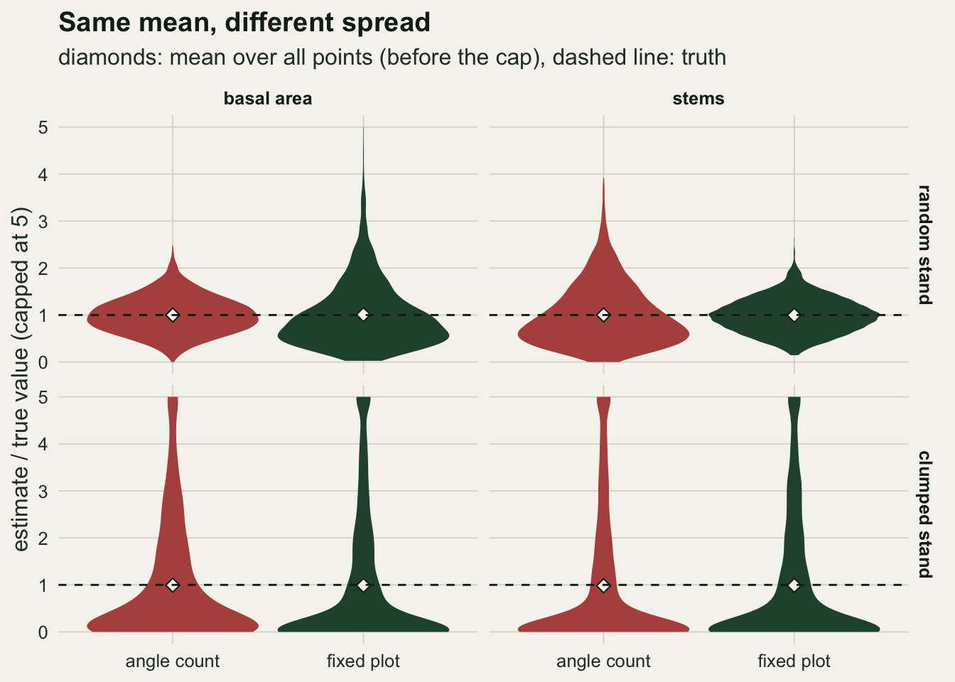
Clumping narrows both gaps
The closed forms assume the stems are placed at random. Real stands are not, and clumping adds count variance that has nothing to do with tree size. Whether it adds that variance equally to both designs is the question, because the angle count looks at a big tree over a big circle and at a small tree over a small one, while the fixed plot uses one circle for all. The sweep below builds eight stands at each of five spatial patterns, the random stand and Thomas clusters with a scatter of 3, 6, 12 and 24 m around the centres, and measures both coefficient of variation ratios on each stand with 2000 points.
sd_grid <- c(NA, 3, 6, 12, 24)
n_stands <- 8
set.seed(2610)
sweep_rows <- list()
for (cs in sd_grid) for (k in seq_len(n_stands)) {
  st <- make_stand(n_ha, cs, rev_j); tr <- stand_truth(st)
  pts <- data.frame(x = runif(n_pts, 0, side_m), y = runif(n_pts, 0, side_m))
  est <- tally(st, pts, baf_set, equal_radius(tr, baf_set))
  cvs <- apply(est, 2, cv_of)
  sweep_rows[[length(sweep_rows) + 1]] <- data.frame(
    clump = ifelse(is.na(cs), "random", sprintf("%g m", cs)),
    ba_ratio = cvs[["ba_fixed"]] / cvs[["ba_angle"]], n_ratio = cvs[["n_angle"]] / cvs[["n_fixed"]],
    th_ba = theory_ba(st), th_n = theory_n(st))
}
sw <- do.call(rbind, sweep_rows)
clump_lev <- c(sprintf("%g m", sd_grid[-1]), "random")
sw$clump <- factor(sw$clump, levels = clump_lev)
agg_fun <- function(v) c(mean = mean(v), se = sd(v) / sqrt(length(v)))
sw_sum <- do.call(rbind, lapply(clump_lev, function(cl) {
  s <- sw[sw$clump == cl, ]
  data.frame(clump = cl, total = c("basal area", "stems"),
             ratio = c(mean(s$ba_ratio), mean(s$n_ratio)),
             se = c(sd(s$ba_ratio), sd(s$n_ratio)) / sqrt(nrow(s)),
             theory = c(mean(s$th_ba), mean(s$th_n)))
}))
sw_sum$clump <- factor(sw_sum$clump, levels = clump_lev)
sr <- function(cl, tot) sw_sum$ratio[sw_sum$clump == cl & sw_sum$total == tot]
sse <- function(cl, tot) sw_sum$se[sw_sum$clump == cl & sw_sum$total == tot]
min_stand_n <- min(sw$n_ratio); min_stand_ba <- min(sw$ba_ratio)
th_ba_rand <- sw_sum$theory[sw_sum$clump == "random" & sw_sum$total == "basal area"]
th_n_rand <- sw_sum$theory[sw_sum$clump == "random" & sw_sum$total == "stems"]
rand <- sw[sw$clump == "random", ]
gap_ba <- rand$th_ba - rand$ba_ratio; gap_n <- rand$th_n - rand$n_ratio
gap_ba_m <- mean(gap_ba); gap_ba_se <- sd(gap_ba) / sqrt(nrow(rand))
gap_n_m <- mean(gap_n); gap_n_se <- sd(gap_n) / sqrt(nrow(rand))
# Welch t for the basal area dip at 6 m and the stem plateau at 3 and 6 m
welch <- function(a, b, v) t.test(sw[[v]][sw$clump == a], sw[[v]][sw$clump == b])$statistic[[1]]
d_ba_3_6 <- sr("3 m", "basal area") - sr("6 m", "basal area"); t_ba_3_6 <- welch("3 m", "6 m", "ba_ratio")
d_ba_12_6 <- sr("12 m", "basal area") - sr("6 m", "basal area"); t_ba_12_6 <- welch("12 m", "6 m", "ba_ratio")
d_n_3_6 <- sr("3 m", "stems") - sr("6 m", "stems"); t_n_3_6 <- welch("3 m", "6 m", "n_ratio")
s24 <- sw[sw$clump == "24 m", ]; i24 <- which.max(s24$ba_ratio)
max24_ba <- s24$ba_ratio[i24]; max24_th <- s24$th_ba[i24]; max_rand_ba <- max(rand$ba_ratio)
With the stems at random, the basal area ratio averages 1.76 (standard error across stands 0.01), a little below its closed form of 1.80 on the same tree lists (a paired gap of 0.04, standard error 0.02), and the stem ratio 1.67 (0.02) sits on its closed form of 1.67 (paired gap 0.005, standard error 0.017). Ordered by the scatter, from tight clusters to none, the basal area ratio is 1.34 at 3 m (standard error 0.009), 1.22 at 6 m (0.013), 1.31 at 12 m (0.017) and 1.61 at 24 m (0.059); the stem ratio is 1.080 (0.005), 1.077 (0.006), 1.18 (0.012) and 1.46 (0.019). No single stand out of the 40 put either ratio below one: the lowest basal area ratio on any stand is 1.16 and the lowest stem ratio 1.04.
So the direction of the textbook result survives clumping and its size does not: every clustered pattern gave a smaller ratio than the random stand for both totals. The two totals do not follow the same shape along the scatter. For basal area the gap is smallest at a 6 m scatter and larger at both 3 and 12 m, by 0.12 and 0.09 over eight stands each (Welch t of 8.0 and 4.3). For stems it sits at the same low level at 3 and 6 m (a difference of 0.003, t of 0.4) and then grows steadily with the scatter towards the random-stand value; eight stands are enough to show that plateau, not to place a minimum inside it. At 24 m, where ten centres per hectare with that much scatter overlap into something nearer to a random stand at the scale of one plot, the basal area ratio also varies most between stands: one stand reached 1.95, above every random stand (the highest of those was 1.82), and its own closed form was 2.13, the mark of a heavy tail of large trees on that tree list. A plausible reading of the overall drop is that the extra variance from where the clusters fall reaches both designs, because both count the trees of whichever cluster the point lands in, so the spread of tree sizes, the only part of the variance that separates the two designs in a random stand, becomes a smaller share of the total.
ggplot(sw_sum, aes(clump, ratio, colour = total, group = total)) +
  geom_hline(yintercept = 1, colour = te_body, linewidth = 0.5) +
  geom_hline(data = data.frame(total = c("basal area", "stems"), th = c(th_ba_rand, th_n_rand)),
             aes(yintercept = th, colour = total), linetype = "dashed", linewidth = 0.6) +
  geom_jitter(data = data.frame(clump = rep(sw$clump, 2), total = rep(c("basal area", "stems"), each = nrow(sw)),
                                ratio = c(sw$ba_ratio, sw$n_ratio)),
              width = 0.12, height = 0, size = 1.1, alpha = 0.45) +
  geom_line(linewidth = 0.9) +
  geom_errorbar(aes(ymin = ratio - 2 * se, ymax = ratio + 2 * se), width = 0.15, linewidth = 0.5) +
  geom_point(size = 2.6) +
  scale_colour_manual(values = c("basal area" = te_rust, "stems" = te_forest), name = NULL,
                      labels = c("basal area: CV fixed / CV angle", "stems: CV angle / CV fixed")) +
  scale_x_discrete(labels = c("3 m", "6 m", "12 m", "24 m", "random\n(no clusters)")) +
  scale_y_continuous(limits = c(0.9, NA)) +
  labs(x = "cluster scatter", y = "ratio of coefficients of variation",
       title = "Clumping shrinks the difference between designs",
       subtitle = "dashed: closed form for a random stand, small dots: single stands") +
  theme_datasheet() + theme(legend.position = "bottom")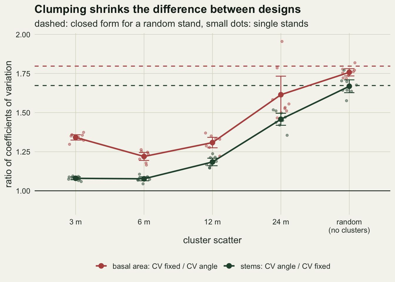
Edges: torus, buffer and slopover
A real stand has a boundary, and a tree near it has part of its inclusion zone outside the stand, where no point will ever be placed. The torus removes that problem by construction. The field alternatives are a buffer, sample points only in an inner region and trees counted wherever they stand, or a correction such as the mirage method. The chunk below takes the clumped stand as a plane with a hard edge and compares three versions on the same stand: the torus, a buffer as wide as the largest limiting distance, and points anywhere in the square with no correction.
buffer_m <- ceiling(max_r_main)
set.seed(2611)
pts_buf <- data.frame(x = runif(n_pts, buffer_m, side_m - buffer_m),
                      y = runif(n_pts, buffer_m, side_m - buffer_m))
est_buf <- tally(st_main, pts_buf, baf_set, r_fix_main, torus = FALSE)
est_buf_torus <- tally(st_main, pts_buf, baf_set, r_fix_main, torus = TRUE)
buf_gap <- max(abs(est_buf - est_buf_torus))
cv_buf <- apply(est_buf, 2, cv_of)
ratio_ba_buf <- cv_buf[["ba_fixed"]] / cv_buf[["ba_angle"]]
ratio_n_buf <- cv_buf[["n_angle"]] / cv_buf[["n_fixed"]]
inner <- st_main$x > buffer_m & st_main$x < side_m - buffer_m &
         st_main$y > buffer_m & st_main$y < side_m - buffer_m
inner_ha <- (side_m - 2 * buffer_m)^2 / 1e4
tr_inner <- c(ba = sum(st_main$g[inner]) / inner_ha, n = sum(inner) / inner_ha)
buf_to_inner <- colMeans(est_buf) / truth_vec(tr_inner)
# slopover: the same points, plane minus torus, so only the edge differs
est_naive <- tally(st_main, pts_main, baf_set, r_fix_main, torus = FALSE)
loss <- sweep(est_naive - est_main, 2, truth_vec(tr_main), "/")
loss_mean <- colMeans(loss); loss_se <- apply(loss, 2, sd) / sqrt(n_pts)
With a buffer of 25 m, at least the largest limiting distance, a point in the inner region never reaches the edge, so its tallies on the plane are the tallies on the torus: the largest difference over the 2000 buffer points is 0. The buffer changes which part of the stand is sampled, not how a point is scored. In this clumped stand the inner 2.25 hectares carry 29.3 square metres of basal area per hectare against 25.4 for the whole square, and the buffer means sit at 1.026 and 1.029 of the inner basal area for the angle count and the fixed plot. The trees in the buffer contribute to points near the inner edge, so the inner-region total is only an approximate target. The coefficient of variation ratios under the buffer are 1.17 for basal area and 1.07 for stems, against 1.20 and 1.06 on the torus, so the comparison between designs does not rest on the edge treatment.
Ignoring the edge altogether is another matter. Scoring the same 2000 points on the plane instead of the torus isolates the slopover loss exactly, point by point. The angle count loses 3.3 per cent of the true basal area (standard error 0.35 percentage points) and 1.3 per cent of the stems (0.21); the fixed plot loses 2.0 per cent of the basal area (0.38) and 1.5 per cent of the stems (0.27). For basal area the angle count loses more, because the inclusion zones of large trees reach up to 24.9 m, where the fixed plot never looks further than 5.12 m, and the trees with the widest zones carry the most basal area. The stem estimate is carried by small trees with small zones, which rarely cross the edge, and its loss is on the scale of the fixed plot’s.
Borderline trees
A tree close to the limiting distance is hard to call with a prism. Say the observer cannot tell in from out within a band of fixed width around the limiting distance, and resolves every tree in the band the same way. Counting them all in adds the trees whose distance lies between R and R plus the band; counting them all out removes those between R minus the band and R. Because the band has a fixed width in metres and R grows with diameter, the band is a larger share of a small tree’s inclusion zone than of a large tree’s, and the relative bias depends on the diameter distribution. An error that is a fixed share of the limiting distance, which is what a slightly wrong gauge angle produces, gives the same relative bias for every tree.
The exact bias follows from the tree list, since each tree’s expected extra contribution is the area of its annulus divided by the area of its inclusion zone, times its weight. The simulation checks that with the paired difference between the biased and the exact tally at the same points. Two stands with random placement and similar basal area are compared: the reverse-J stand from above, and a mature stand with 260 stems per hectare and diameters of seven centimetres plus a lognormal with a median of 26 cm and a log standard deviation of 0.35.
tol_grid <- c(0.05, 0.10, 0.20, 0.30)          # band half-width, metres
eps_share <- 0.01                              # error as a share of the limiting distance
mature <- function(n) 7 + rlnorm(n, log(26), 0.35)
set.seed(2612)
st_mat <- make_stand(260, NA, mature); tr_mat <- stand_truth(st_mat)
exact_bias <- function(st, tol, rule) {
  r2 <- lim_dist(st$dbh, baf_set)^2
  shift <- if (rule == "in") pmin(2 * tol * sqrt(r2) + tol^2, Inf) else
             -pmin(r2, 2 * tol * sqrt(r2) - tol^2)
  c(ba = sum(shift) / sum(r2), n = mean(shift / r2))
}
sim_bias <- function(st, tr, pts, tols) {
  r_lim <- lim_dist(st$dbh, baf_set); w_n <- baf_set / st$g
  acc <- array(0, c(nrow(pts), length(tols), 4))
  for (s in seq(1, nrow(pts), by = 200)) {
    ii <- s:min(nrow(pts), s + 199)
    dd <- dist_block(pts$x[ii], pts$y[ii], st, TRUE)
    base <- sweep(dd, 2, r_lim, "<")
    for (j in seq_along(tols)) {
      add <- sweep(dd, 2, r_lim + tols[j], "<") & !base
      drop <- base & !sweep(dd, 2, r_lim - tols[j], "<")
      acc[ii, j, 1] <- baf_set * rowSums(add);  acc[ii, j, 2] <- add %*% w_n
      acc[ii, j, 3] <- -baf_set * rowSums(drop); acc[ii, j, 4] <- -(drop %*% w_n)
    }
  }
  scale_by <- c(tr[["ba"]], tr[["n"]], tr[["ba"]], tr[["n"]])
  mean_rel <- sweep(apply(acc, c(2, 3), mean), 2, scale_by, "/")
  se_rel <- sweep(apply(acc, c(2, 3), sd) / sqrt(nrow(pts)), 2, scale_by, "/")
  list(mean = mean_rel, se = se_rel)
}
pts_b <- data.frame(x = runif(n_pts, 0, side_m), y = runif(n_pts, 0, side_m))
stands_b <- list("reverse-J stand" = list(st = st_csr, tr = tr_csr),
                 "mature stand" = list(st = st_mat, tr = tr_mat))
border_rows <- list(); sim_rows <- list()
for (nm in names(stands_b)) {
  sb <- stands_b[[nm]]
  tol_fine <- seq(0, 0.3, by = 0.01)
  for (rule in c("in", "out")) {
    ex <- t(vapply(tol_fine, function(tl) exact_bias(sb$st, tl, rule), numeric(2)))
    border_rows[[length(border_rows) + 1]] <- data.frame(
      stand = nm, rule = sprintf("all counted %s", rule), tol = rep(tol_fine, 2),
      total = rep(c("basal area", "stems"), each = length(tol_fine)), bias = c(ex[, 1], ex[, 2]))
  }
  sb_sim <- sim_bias(sb$st, sb$tr, pts_b, tol_grid)
  sim_rows[[nm]] <- data.frame(
    stand = nm, tol = rep(tol_grid, 4),
    rule = rep(c("all counted in", "all counted in", "all counted out", "all counted out"), each = length(tol_grid)),
    total = rep(c("basal area", "stems", "basal area", "stems"), each = length(tol_grid)),
    bias = as.vector(sb_sim$mean), se = as.vector(sb_sim$se))
}
bord <- do.call(rbind, border_rows); bsim <- do.call(rbind, sim_rows)
bsim$exact <- mapply(function(nm, tl, rl, tot) {
  e <- exact_bias(stands_b[[nm]]$st, tl, ifelse(rl == "all counted in", "in", "out"))
  e[[ifelse(tot == "basal area", "ba", "n")]]
}, bsim$stand, bsim$tol, bsim$rule, bsim$total)
z_border <- max(abs(bsim$bias - bsim$exact) / bsim$se)
eb <- function(nm, tl, rule, tot) exact_bias(stands_b[[nm]]$st, tl, rule)[[tot]]
half_ba <- (eb("reverse-J stand", 0.1, "in", "ba") + eb("reverse-J stand", 0.1, "out", "ba")) / 2
eps_bias <- 2 * eps_share + eps_share^2
dbh_mean_rj <- mean(st_csr$dbh); dbh_mean_mat <- mean(st_mat$dbh)
The mature stand has 270 stems per hectare and 27.7 square metres of basal area per hectare, with a mean diameter of 34.6 cm against 18.4 cm in the reverse-J stand. Simulated and exact biases agree within 1.82 Monte Carlo standard errors at every band, rule, total and stand.
With a band of 10 cm and every borderline tree counted in, basal area is overestimated by 3.2 per cent in the reverse-J stand and by 2.1 per cent in the mature stand. The stem density estimate from the same count is 5.8 per cent too high in the reverse-J stand and 2.5 per cent in the mature stand, because the small trees that carry the largest stem weights are also the ones with the band taking the largest share of their zone. Counting all borderline trees out gives nearly the mirror image, underestimates of 3.1 and 2.1 per cent for basal area. Calling half the band in and half out leaves an expected basal area bias of 0.034 per cent in the reverse-J stand at the same band. At a 30 cm band the in rule reaches 9.8 per cent for basal area and 17.9 per cent for stems in the reverse-J stand.
The proportional error behaves differently. If every limiting distance is judged 1 per cent too long, the relative bias is 2.01 per cent for basal area and for stems, in both stands, whatever the diameters.
bord$stand <- factor(bord$stand, levels = names(stands_b))
bsim$stand <- factor(bsim$stand, levels = names(stands_b))
ggplot(bord, aes(100 * tol, 100 * bias, colour = stand, linetype = rule)) +
  geom_hline(yintercept = 0, colour = te_body, linewidth = 0.4) +
  geom_line(linewidth = 0.9) +
  geom_errorbar(data = bsim, aes(ymin = 100 * (bias - 2 * se), ymax = 100 * (bias + 2 * se)),
                width = 0.8, linewidth = 0.4, linetype = "solid") +
  geom_point(data = bsim, size = 1.9) +
  facet_wrap(~ total) +
  scale_colour_manual(values = c("reverse-J stand" = te_rust, "mature stand" = te_forest), name = NULL) +
  scale_linetype_manual(values = c("all counted in" = "solid", "all counted out" = "dashed"), name = NULL) +
  labs(x = "half-width of the borderline band (cm)", y = "relative bias (per cent)",
       title = "Borderline bias depends on the diameters",
       subtitle = "same band, two stands, two totals") +
  guides(colour = guide_legend(nrow = 1), linetype = guide_legend(nrow = 1)) +
  theme_datasheet() +
  theme(legend.position = "bottom", legend.box = "vertical",
        strip.text = element_text(colour = te_ink, face = "bold"))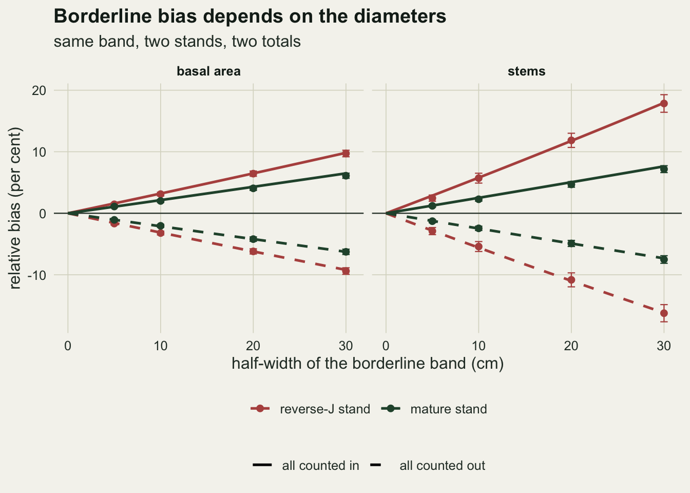
What to report
Give the gauge and its factor, and the minimum diameter. The BAF fixes the limiting distance of every tree and the calliper threshold decides which small trees can enter the stem estimate at all; a stem density from an angle count means nothing without both.
When stem density comes from an angle count, report its coefficient of variation separately from that of basal area, computed from the per-point stem estimates. Quoting the basal area precision for both totals is the easy mistake, and in the random stand above the stem coefficient of variation was 1.65 times the basal area one from the same points.
Say how borderline trees were resolved. If they were measured, give the distance and diameter precision; if they were called by eye with a rule, say which rule. A band of fixed width is not a fixed percentage bias, and the correction a reader would apply depends on the stand and on the gauge’s BAF.
State the edge treatment. A buffer, a mirage or walkthrough correction, or a boundary that nobody sampled near are different designs, and uncorrected slopover biased the angle count estimate of basal area downwards by more than the fixed plot estimate in the stand above.
Honest limits
The stands are simulated, and size is independent of position within them. In a real stand small trees gather in gaps and under canopy openings and large trees space themselves out, which couples diameter and clustering in exactly the way that could move the coefficient of variation ratios above or below the values measured here. The sweep also used one diameter distribution and one BAF; the closed forms show that the random-stand ratios depend only on the spread of tree sizes, not on the BAF, but that claim was checked in the clumped stands only in an unreported pilot run, not in a chunk here. Only one cluster density was tried, and a 3 m scatter packs a cluster centre far denser than any real stand.
Equal effort was defined as equal expected trees per point. Field time depends on walking between points, on how many diameters are taken and on borderline checks, and on that accounting the angle count for basal area alone is cheaper than the definition here gives it credit for. A cost-based comparison would change the numbers, and it was not run.
The coefficients of variation are design-based, over points within one stand, and a cruise of n points divides them by the square root of n when the points are placed independently at random. On a systematic grid in a clumped stand that no longer holds, and the variance estimator would need the same care as in any other spatial survey.
The borderline model is a sharp band resolved one way. Real observers are inconsistent: some trees in the band go in and some out, and a half-and-half rule is close to unbiased in expectation, as the section above shows, while adding its own noise. The simulation does not model the observer, only the two extreme rules and a proportional error, which bracket what a consistent observer can do.
Finally, the torus is an idealisation. The buffer comparison shows it does not drive the design comparison, but a buffer throws away the outer part of a small stand, and the mirage and walkthrough corrections that keep it were not simulated.
References
Grosenbaugh LR 1952 Journal of Forestry 50(1):32-37 (10.1093/jof/50.1.32)
Horvitz DG, Thompson DJ 1952 Journal of the American Statistical Association 47(260):663-685 (10.1080/01621459.1952.10483446)
Gregoire TG, Valentine HT 2008 Sampling Strategies for Natural Resources and the Environment (ISBN 978-1-58488-370-8)