library(ggplot2); library(MASS)
theme_te <- function() {
  theme_minimal(base_size = 12) +
    theme(
          plot.background  = element_rect(fill = "#f5f4ee", colour = NA),
          panel.background = element_rect(fill = "#f5f4ee", colour = NA),
          panel.grid.minor = element_blank(),
          panel.grid.major = element_line(colour = "#e7e6da", linewidth = 0.3),
          plot.title = element_text(colour = "#16241d", face = "bold", size = 13),
          plot.subtitle = element_text(colour = "#5d6b61", size = 10),
          axis.title = element_text(colour = "#46604a"),
          axis.text = element_text(colour = "#5d6b61"),
          legend.title = element_text(colour = "#46604a"),
          legend.text = element_text(colour = "#5d6b61"))
}
pal_forest <- "#275139"; pal_gold <- "#cda23f"; pal_rust <- "#b5534e"

grts_address <- function(x, y, L = 8L) {
  n <- length(x); addr <- numeric(n)
  recurse <- function(idx, xlo, xhi, ylo, yhi, level, prefix) {
    if (level >= L || length(idx) <= 1L) { addr[idx] <<- prefix * 4^(L - level); return(invisible(NULL)) }
    xm <- (xlo + xhi)/2; ym <- (ylo + yhi)/2
    q <- (x[idx] >= xm) + 2L*(y[idx] >= ym); perm <- sample(0:3)
    for (qq in 0:3) {
      sub <- idx[q == qq]; if (length(sub) == 0L) next
      cxlo <- if (qq %% 2L == 1L) xm else xlo; cxhi <- if (qq %% 2L == 1L) xhi else xm
      cylo <- if (qq >= 2L) ym else ylo;       cyhi <- if (qq >= 2L) yhi else ym
      recurse(sub, cxlo, cxhi, cylo, cyhi, level + 1L, prefix*4 + perm[qq + 1L])
    }
  }
  recurse(seq_len(n), 0, 1, 0, 1, 0L, 0); addr
}
grts_draw <- function(x, y, m, pip = NULL, L = 8L) {
  n <- length(x); if (is.null(pip)) pip <- rep(m/n, n)
  a <- grts_address(x, y, L); ord <- order(a, runif(n))
  cs <- cumsum(pip[ord]); picks <- runif(1) + 0:(m - 1)
  ord[findInterval(picks, c(0, cs), rightmost.closed = TRUE)]
}

set.seed(404)
side <- 22
g <- expand.grid(x = seq(0.02, 0.98, length.out = side),
                 y = seq(0.02, 0.98, length.out = side))
N <- nrow(g)
blob <- exp(-((g$x - 0.72)^2 + (g$y - 0.30)^2) / 0.02)
rare <- blob > quantile(blob, 0.88)                    # about a tenth of the frame
y <- rnorm(N, ifelse(rare, 14, 9), ifelse(rare, 2.2, 1.2))
mu_true  <- mean(y)
frac_rare <- mean(rare)
m <- 40Unequal-probability spatial sampling
R
survey design
spatial statistics
monitoring
ecology tutorial
Oversampling a rare habitat with GRTS, and why the plain sample mean is then biased. The Horvitz-Thompson estimator for unequal inclusion probabilities in R.
Equal-probability sampling treats every place the same. Often you do not want that. A rare wetland class covers a tenth of the park but carries most of the conservation interest; a few large lakes hold most of the water; some strata are cheap to reach and some are not. In all of these you want to visit some units more often than others, which means giving them a higher inclusion probability. GRTS handles unequal probabilities without any change to the machinery, because the draw already lays the inclusion probabilities along the space-filling order and takes a systematic pick. The subtlety is on the analysis side: once the probabilities differ, the plain sample mean is biased, and you have to weight by the inclusion probability to get an honest answer.
A rare class worth oversampling
Take a landscape with a small patch of a rare habitat class that has both a higher mean value and more variability than the common matrix around it. Under equal-probability sampling the patch gets its fair share of sites, which for a rare class is very few, so any estimate specific to that class is noisy.
Setting unequal inclusion probabilities
To oversample the rare class we give its units a higher inclusion density. Here they get four times the base density of the common class. The probabilities are then scaled so they still sum to the sample size, and capped below one. GRTS turns those probabilities into a spread-out sample exactly as before; the only change is the vector we feed it.
w <- ifelse(rare, 4, 1)
pip <- m * w / sum(w)
pip <- pmin(pip, 0.999)
pip <- m * pip / sum(pip)                              # keep sum(pip) = m after capping

set.seed(4041)
samp <- grts_draw(g$x, g$y, m, pip = pip)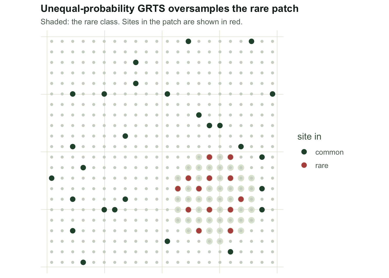
The plain mean is now biased
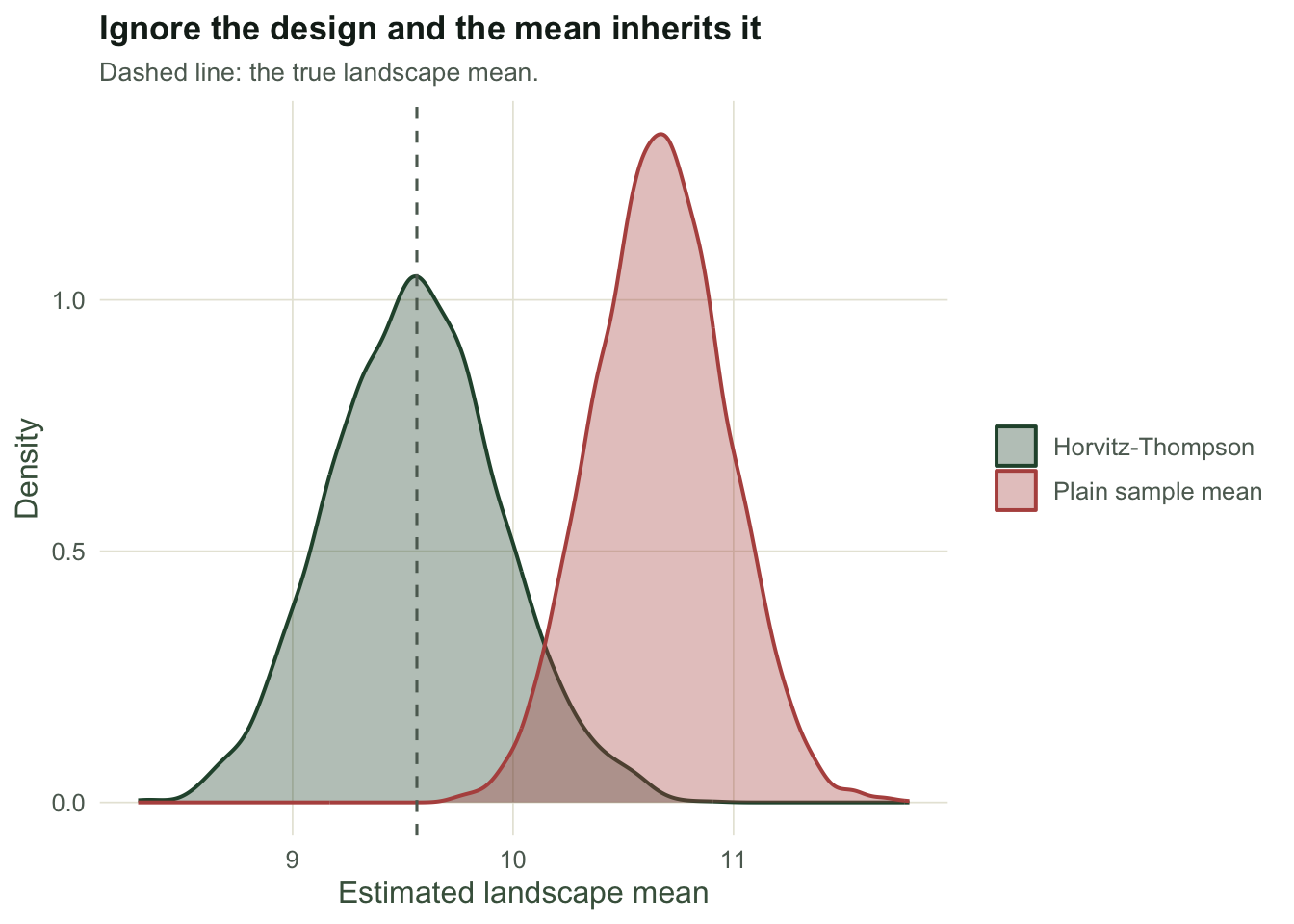
The oversampling works: instead of the handful of rare sites an equal-probability survey would return, the unequal design puts many more inside the patch. But the rare class has a higher mean, so a sample that overrepresents it will overshoot the landscape average. The plain sample mean is no longer an honest estimate of anything. The Horvitz-Thompson mean, which divides each observation by its inclusion probability before averaging, undoes the overrepresentation.
set.seed(505)
R <- 4000
n_rare_eq <- integer(R); n_rare_un <- integer(R)
plain <- numeric(R); ht <- numeric(R)
for (r in seq_len(R)) {
  se <- grts_draw(g$x, g$y, m)                        # equal probability
  su <- grts_draw(g$x, g$y, m, pip = pip)             # unequal probability
  n_rare_eq[r] <- sum(rare[se]); n_rare_un[r] <- sum(rare[su])
  plain[r] <- mean(y[su])                             # ignores the design
  ht[r]    <- sum(y[su] / pip[su]) / N                # Horvitz-Thompson mean
}
rare_eq <- mean(n_rare_eq); rare_un <- mean(n_rare_un)
bias_plain <- mean(plain) - mu_true
bias_ht    <- mean(ht)    - mu_true
An equal-probability survey lands 4.8 sites in the rare class on average; the unequal design lands 14.1, so the small patch is now well covered. The cost is that the plain sample mean overestimates the landscape average by +1.099, because the rare high-value class is overrepresented. The Horvitz-Thompson mean removes exactly that bias: its average error is +0.003, effectively zero. The rule is simple and unforgiving. As soon as inclusion probabilities differ, weight by the reciprocal of the inclusion probability, or your estimate inherits the design.
What you actually gain, and what you do not
The reason to accept that extra bookkeeping is coverage. The quantity that improves under oversampling is the estimate specific to the rare class, because it now rests on many sites instead of a handful.
set.seed(606)
est_rare_eq <- numeric(R); est_rare_un <- numeric(R)
for (r in seq_len(R)) {
  se <- grts_draw(g$x, g$y, m); su <- grts_draw(g$x, g$y, m, pip = pip)
  est_rare_eq[r] <- if (any(rare[se])) mean(y[se][rare[se]]) else NA
  est_rare_un[r] <- if (any(rare[su])) mean(y[su][rare[su]]) else NA
}
sd_rare_eq <- sd(est_rare_eq, na.rm = TRUE)
sd_rare_un <- sd(est_rare_un, na.rm = TRUE)
The standard deviation of the rare-class mean drops from 0.888 under equal probability to 0.466 under the oversampled design, close to half. That is the payoff: a usable estimate for the class you cared about.
What unequal probability does not buy is a free reduction in the variance of the overall mean. Oversampling one class means undersampling the rest, and the Horvitz-Thompson weights that put things right also inflate the variance of any observation with a small inclusion probability. Unequal probability pays off for the overall estimate only when the inclusion probabilities are close to proportional to the values themselves, the classical case of sampling with probability proportional to size when estimating a total. Choose unequal probabilities to guarantee coverage or to follow a size measure, not in the hope of a tighter landscape average for nothing.
References
Horvitz DG, Thompson DJ 1952 Journal of the American Statistical Association 47(260):663-685 (10.1080/01621459.1952.10483446)
Stevens DL, Olsen AR 2004 Journal of the American Statistical Association 99(465):262-278 (10.1198/016214504000000250)
Sarndal CE, Swensson B and Wretman J 1992 Model Assisted Survey Sampling. Springer, New York; softcover printing 2003, ISBN 978-0-387-40620-6.