library(ggplot2)
library(patchwork)

te_paper  <- "#f5f4ee"
te_ink    <- "#16241d"
te_body   <- "#2c3a31"
te_forest <- "#275139"
te_rust   <- "#b5534e"
te_gold   <- "#c9b458"
te_line   <- "#dad9ca"

theme_datasheet <- function() {
  theme_minimal(base_size = 12) +
    theme(plot.background  = element_rect(fill = te_paper, colour = NA),
          panel.background = element_rect(fill = te_paper, colour = NA),
          panel.grid.major = element_line(colour = te_line, linewidth = 0.3),
          panel.grid.minor = element_blank(),
          text             = element_text(colour = te_body),
          plot.title       = element_text(colour = te_ink, face = "bold"),
          plot.subtitle    = element_text(colour = te_body),
          axis.text        = element_text(colour = te_body))
}Design weights in a stratified regression
R
survey design
stratified sampling
regression
simulation
ecology tutorial
A design weight is compulsory for a stratified mean but optional for a regression slope. Measuring in R what it costs, what it fixes, and the test that decides.
An upland survey maps twenty thousand grassland cells and draws three hundred plots from them. Spring-fed flushes cover a small share of the map, but they hold the orchids the survey was funded for, so the design sends two plots in five into the flushes and the rest onto the ordinary slopes. Every plot records a soil moisture index and the log of the above-ground biomass of the sward, and the analysis the report needs is the slope of log biomass on moisture across the whole landscape. The flushes are wetter than the slopes, so the oversampled stratum also sits at one end of the covariate.
The design weight for a plot is the number of cells its stratum holds divided by the number of plots drawn from it. For the landscape mean of log biomass that weight is compulsory: leave it out and the mean inherits the oversampling. For the slope the answer is different, and it has been known for a long time. DuMouchel and Duncan showed in 1983 that in a stratified sample the weighted and the unweighted regression estimate the same coefficient when the model is right, that the unweighted fit is then the more precise, and that the difference between the two fits is a specification test. Solon, Haider and Wooldridge restated the whole question in 2015 for applied work: a weight is needed to recover the population coefficient when the effect differs across the groups the design treated unequally (and they would rather that heterogeneity were modelled), or when selection depends on the response itself, and they recommend comparing the weighted and unweighted fits as a check. None of this is new, and this post is a demonstration of those papers rather than a finding of its own. What it measures is the price of the weight when it is not needed, the bias it removes when it is, and how well the gap between the two fits tells those cases apart.
The nearest post on this site is Transporting an effect to a new region, which reweights a sample towards a target population’s covariate distribution and charges the variance for it in “The price”. That post pays for moving an answer to a new population; this one asks whether a slope needs the weight at all, and answers with a test rather than a rule. On this site a design weight almost always stands in front of a mean or a total. One place where an inverse-probability weight enters a regression coefficient is GPS fix loss and the collars you drop, and there it is needed even with the model right, because fix loss depends on canopy and thins only the used points, which are the response of the selection model: the second of Solon, Haider and Wooldridge’s cases. Unequal-probability spatial sampling shows the plain mean going wrong when a rare class is oversampled, and Stratified random sampling in ecology and Checking a stratified design stay with the stratified mean and its variance. Propensity scores and IPW prints Kish’s effective sample size for a set of weights, and one section below checks what that number says about a slope.
A rare habitat, oversampled
The landscape is simulated so that the truth is known. Each cell is a flush with probability 0.08, and the moisture index is standard normal on the slopes and shifted up by 1.2 in the flushes. Log biomass is a line in moisture plus normal noise with a standard deviation of 1.5, and three versions of the truth are used below: one where the line is the same everywhere, one where the flushes have a steeper slope, and one where biomass curves in moisture. The target throughout is the census slope: the least squares slope fitted to all twenty thousand cells of the realised landscape, which is the number a surveyor who could measure every cell would report.
Each sample is a stratified random sample without replacement, a fixed number of plots from each stratum. Both fits are computed by hand, and so is the variance of their difference. That variance is the stratified linearisation: every plot contributes an influence term to each slope, the difference of the two terms is summed within strata, and the usual stratified variance of a total is applied to it. It is written two ways, with the finite population correction and without it, because the two answer slightly different questions and the difference turns out to matter.
n_cell    <- 20000L
p_rare    <- 0.08
x_shift   <- 1.2
sigma_e   <- 1.5
n_plot    <- 300L
n_rare    <- 120L
slope_gap <- 0.9
curv_q    <- 0.45

make_landscape <- function(truth, shift = x_shift, gap = slope_gap) {
  rare <- rbinom(n_cell, 1L, p_rare)
  x    <- rnorm(n_cell, mean = shift * rare, sd = 1)
  mu   <- switch(truth,
    right     = 1 + 1.0 * x,
    by_strat  = 1 + (1.0 + gap * rare) * x,
    curvature = 1 + 1.0 * x + curv_q * x^2)
  list(x = x, y = mu + rnorm(n_cell, 0, sigma_e), rare = rare)
}
census_slope <- function(land) cov(land$x, land$y) / var(land$x)

# sums over the whole map, used to average a stratum-wise fit over every cell
map_moments <- function(land) {
  xc   <- land$x - mean(land$x)
  in_r <- land$rare == 1L
  c(sr1 = sum(xc[in_r]), sr2 = sum(land$x[in_r] * xc[in_r]),
    sc1 = sum(xc[!in_r]), sc2 = sum(land$x[!in_r] * xc[!in_r]), sxx = sum(xc^2))
}

fit_pair <- function(land, idx_r, idx_c, n_r, n_c, mom = NULL) {
  pick <- c(idx_r[sample.int(length(idx_r), n_r)],
            idx_c[sample.int(length(idx_c), n_c)])
  xs <- land$x[pick]; ys <- land$y[pick]
  in_r  <- rep(c(TRUE, FALSE), c(n_r, n_c))
  big_r <- length(idx_r); big_c <- length(idx_c)
  wt <- ifelse(in_r, big_r / n_r, big_c / n_c)
  xm <- cbind(1, xs)
  a_u <- crossprod(xm); a_w <- crossprod(xm, xm * wt)
  b_u <- solve(a_u, crossprod(xm, ys)); b_w <- solve(a_w, crossprod(xm, ys * wt))
  e_u <- as.vector(ys - xm %*% b_u); e_w <- as.vector(ys - xm %*% b_w)
  # influence of each plot on each slope, and on their difference
  inf_u <- solve(a_u, t(xm * e_u))[2, ]
  inf_w <- solve(a_w, t(xm * e_w * wt))[2, ]
  gap_i <- inf_u - inf_w
  s2_r <- var(gap_i[in_r]); s2_c <- var(gap_i[!in_r])
  v_fpc <- n_r * (1 - n_r / big_r) * s2_r + n_c * (1 - n_c / big_c) * s2_c
  v_wr  <- n_r * s2_r + n_c * s2_c
  gap_b <- b_u[2] - b_w[2]
  b_proj <- NA_real_
  if (!is.null(mom)) {
    # separate line per stratum, then the census slope of its predictions
    cf <- lm.fit(cbind(1, xs, in_r, xs * in_r), ys)$coefficients
    b_proj <- ((cf[1] + cf[3]) * mom[["sr1"]] + (cf[2] + cf[4]) * mom[["sr2"]] +
               cf[1] * mom[["sc1"]] + cf[2] * mom[["sc2"]]) / mom[["sxx"]]
  }
  c(b_u = b_u[2], b_w = b_w[2],
    z_fpc = gap_b / sqrt(v_fpc), z_wr = gap_b / sqrt(v_wr),
    m_u = mean(ys), m_w = sum(wt * ys) / sum(wt), b_proj = unname(b_proj))
}
z_crit <- qnorm(0.975)
One landscape with a steeper slope in the flushes shows what the choice looks like on a single survey.
set.seed(3101)
land_scene <- make_landscape("by_strat")
idx_r_s <- which(land_scene$rare == 1L); idx_c_s <- which(land_scene$rare == 0L)
pick_s  <- c(idx_r_s[sample.int(length(idx_r_s), n_rare)],
             idx_c_s[sample.int(length(idx_c_s), n_plot - n_rare)])
plots_s <- data.frame(x = land_scene$x[pick_s], y = land_scene$y[pick_s],
                      rare = land_scene$rare[pick_s])
wt_r_s <- length(idx_r_s) / n_rare
wt_c_s <- length(idx_c_s) / (n_plot - n_rare)
plots_s$wt <- ifelse(plots_s$rare == 1L, wt_r_s, wt_c_s)
fit_u_s <- lm(y ~ x, data = plots_s)
fit_w_s <- lm(y ~ x, data = plots_s, weights = wt)
b_census_s <- census_slope(land_scene)
a_census_s <- mean(land_scene$y) - b_census_s * mean(land_scene$x)
b_u_s <- unname(coef(fit_u_s)[2]); b_w_s <- unname(coef(fit_w_s)[2])
share_r     <- length(idx_r_s) / n_cell
share_plots <- n_rare / n_plot
over_ratio  <- share_plots / share_r
In this landscape the flushes are 8.0 per cent of the cells and 40 per cent of the plots, an oversampling of 5.0 times. A flush plot carries a weight of 13.4 cells and a slope plot 102.2. The census slope is 1.159. The unweighted fit to the three hundred plots gives 1.501 and the weighted fit 1.115.
line_df <- data.frame(
  fit = factor(c("census, all cells", "unweighted plots", "weighted plots"),
               levels = c("census, all cells", "unweighted plots", "weighted plots")),
  a = c(a_census_s, coef(fit_u_s)[1], coef(fit_w_s)[1]),
  b = c(b_census_s, b_u_s, b_w_s))
plots_s$stratum <- ifelse(plots_s$rare == 1L, "flush (oversampled)", "slope")

ggplot(plots_s, aes(x, y)) +
  geom_point(aes(shape = stratum), colour = te_body, alpha = 0.55, size = 1.8) +
  geom_abline(data = line_df, aes(intercept = a, slope = b, colour = fit,
                                  linetype = fit), linewidth = 1) +
  scale_colour_manual(values = c(te_ink, te_rust, te_forest), name = NULL) +
  scale_linetype_manual(values = c("dashed", "solid", "solid"), name = NULL) +
  scale_shape_manual(values = c(17, 1), name = NULL) +
  labs(x = "soil moisture index", y = "log biomass",
       title = "The oversampled flushes pull the plain fit",
       subtitle = "dashed: the census slope the survey is meant to report") +
  theme_datasheet() +
  theme(legend.position = "bottom", legend.box = "vertical")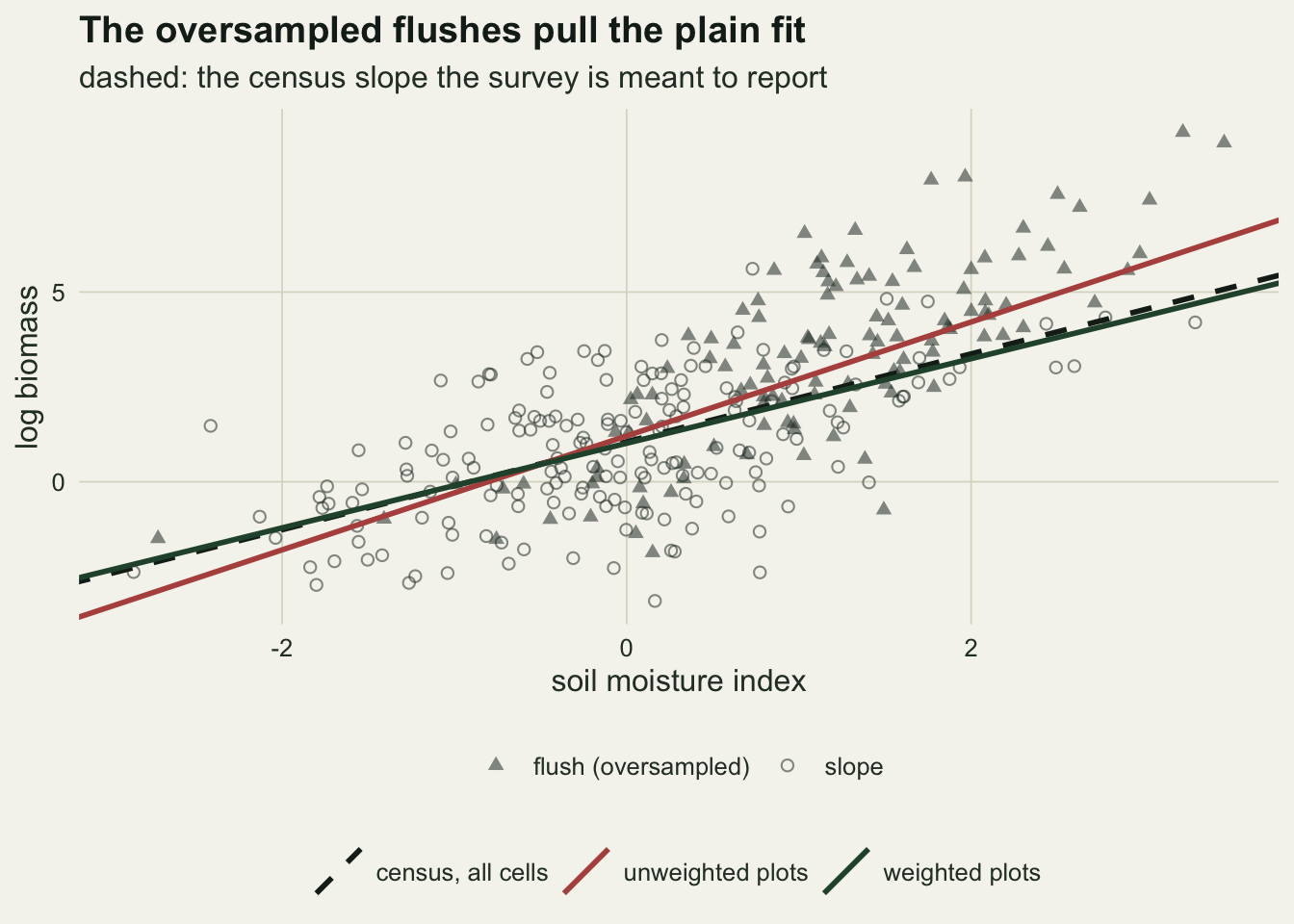
Four truths, two fits
One survey proves nothing, so the comparison is repeated. Four truths are run: the model right, a slope that is 0.9 steeper in the flushes, a curve in moisture with the flushes at the wet end, and the same curve with the flushes moved to the dry end. For each truth there are five fresh landscapes and one thousand stratified samples from each. A third estimator rides along and is discussed in its own section below. Bias is expressed as a share of the census slope itself.
n_land <- 5L
n_rep  <- 1000L
truth_set <- data.frame(
  label = c("model right", "slope differs by stratum",
            "curvature, flushes wet", "curvature, flushes dry"),
  truth = c("right", "by_strat", "curvature", "curvature"),
  shift = c(x_shift, x_shift, x_shift, -x_shift))

set.seed(3102)
truth_out <- do.call(rbind, lapply(seq_len(nrow(truth_set)), function(j) {
  do.call(rbind, lapply(seq_len(n_land), function(k) {
    land  <- make_landscape(truth_set$truth[j], shift = truth_set$shift[j])
    b_pop <- census_slope(land)
    idx_r <- which(land$rare == 1L); idx_c <- which(land$rare == 0L)
    mom   <- map_moments(land)
    draws <- replicate(n_rep, fit_pair(land, idx_r, idx_c, n_rare,
                                       n_plot - n_rare, mom))
    data.frame(label = truth_set$label[j], land = k, census = b_pop,
               bias_u = mean(draws["b_u", ]) - b_pop,
               bias_w = mean(draws["b_w", ]) - b_pop,
               bias_p = mean(draws["b_proj", ]) - b_pop,
               se_bias_w = sd(draws["b_w", ]) / sqrt(n_rep),
               ratio_w = var(draws["b_w", ]) / var(draws["b_u", ]),
               ratio_p = var(draws["b_proj", ]) / var(draws["b_u", ]),
               ratio_m = var(draws["m_w", ]) / var(draws["m_u", ]),
               rej_fpc = mean(abs(draws["z_fpc", ]) > z_crit),
               rej_wr  = mean(abs(draws["z_wr", ]) > z_crit))
  }))
}))
truth_out$pct_u <- 100 * truth_out$bias_u / truth_out$census
truth_out$pct_w <- 100 * truth_out$bias_w / truth_out$census
truth_out$pct_p <- 100 * truth_out$bias_p / truth_out$census

by_truth <- function(col, fun) {
  unname(tapply(truth_out[[col]], truth_out$label, fun)[truth_set$label])
}
census_med <- by_truth("census", median)
pct_u_med <- by_truth("pct_u", median)
pct_u_min <- by_truth("pct_u", min)
pct_u_max <- by_truth("pct_u", max)
abs_w_max <- by_truth("bias_w", function(v) max(abs(v)))
se_w_max  <- max(truth_out$se_bias_w)
wrong     <- truth_out$label != "model right"
abs_w_wrong <- max(abs(truth_out$bias_w[wrong]))
pct_w_wrong <- max(abs(truth_out$pct_w[wrong]))
rej_wrong_min <- min(truth_out$rej_fpc[wrong])
With the model right the census slope is 0.999 (median over landscapes), and both fits are centred on it: the unweighted bias runs from -1.4 to +2.0 per cent of the census slope across the five landscapes, and the weighted bias never exceeds 0.0046 in slope units. The small unweighted offsets are not noise in the samples; they are a property of each finite landscape, and they come back in the section on the test.
With the model wrong the picture splits. When the flushes have the steeper slope, the unweighted fit overshoots the census slope by 28.6 to 31.1 per cent of its value. With the curve and the flushes at the wet end it overshoots by 26.3 to 30.9 per cent; with the flushes moved to the dry end the same curve makes it undershoot, by 36.1 to 40.5 per cent. The sign of the curvature bias belongs to the direction of the covariate shift, not to the curvature. Across all 15 misspecified landscapes the weighted bias never exceeds 0.0078 in slope units, or 0.77 per cent of the census slope, against a Monte Carlo standard error of each landscape’s mean of at most 0.0043.
The mechanism is the one DuMouchel and Duncan wrote down. Least squares fits the best straight line under whatever covariate distribution it is given. The weighted fit is given the landscape’s distribution, rebuilt from the sample, so it targets the census line. The unweighted fit is given the sample’s distribution, in which the wet flushes count 5.0 times over, so it targets the best line for a landscape that is two fifths flush. When the truth is a single straight line those two best lines are the same line; when it is not, they part, and the unweighted fit converges to the wrong one however many plots are added.
bias_long <- rbind(
  data.frame(label = truth_out$label, pct = truth_out$pct_u, est = "unweighted"),
  data.frame(label = truth_out$label, pct = truth_out$pct_w, est = "weighted"),
  data.frame(label = truth_out$label, pct = truth_out$pct_p, est = "stratum lines, averaged over the map"))
bias_long$label <- factor(bias_long$label, levels = rev(truth_set$label))
bias_long$est <- factor(bias_long$est, levels = c("unweighted", "weighted",
                                                  "stratum lines, averaged over the map"))

ggplot(bias_long, aes(pct, label, colour = est)) +
  geom_vline(xintercept = 0, colour = te_body, linewidth = 0.5) +
  geom_point(position = position_dodge(width = 0.6), size = 2.2, alpha = 0.85) +
  scale_colour_manual(values = c(te_rust, te_forest, te_gold), name = NULL) +
  labs(x = "bias, per cent of the census slope", y = NULL,
       title = "The weight matters only when the model is wrong",
       subtitle = "five landscapes per truth, one thousand samples each") +
  theme_datasheet() +
  theme(legend.position = "bottom")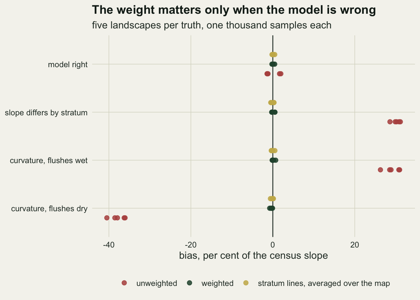
The price when the model is right
When the model is right the weight repairs nothing, and it still costs precision. The price is the ratio of the variance of the weighted slope to the variance of the unweighted one, over repeated samples from the same landscape. The survey reflex is to predict that price from the weights alone, with Kish’s design effect: the number of plots times the sum of the squared weights, divided by the square of the summed weights. That arithmetic is built for a mean. For a slope the variance also depends on where each stratum sits on the covariate, and the same sandwich that gives the test its variance predicts the price from the second moments of moisture in each stratum.
kish_deff <- function(big_r, big_c, n_r, n_c) {
  (n_r + n_c) * (big_r^2 / n_r + big_c^2 / n_c) / (big_r + big_c)^2
}
# design variance of each slope from the stratum moments of the covariate
slope_price <- function(land, n_r, n_c, fpc = TRUE) {
  in_r  <- land$rare == 1L
  big_r <- sum(in_r); big_c <- sum(!in_r)
  f_r <- if (fpc) n_r / big_r else 0; f_c <- if (fpc) n_c / big_c else 0
  m_r <- crossprod(cbind(1, land$x[in_r])) / big_r
  m_c <- crossprod(cbind(1, land$x[!in_r])) / big_c
  inv_u <- solve(n_r * m_r + n_c * m_c)
  inv_w <- solve(big_r * m_r + big_c * m_c)
  v_u <- n_r * (1 - f_r) * (inv_u %*% m_r %*% inv_u)[2, 2] +
         n_c * (1 - f_c) * (inv_u %*% m_c %*% inv_u)[2, 2]
  v_w <- n_r * (1 - f_r) * (big_r / n_r)^2 * (inv_w %*% m_r %*% inv_w)[2, 2] +
         n_c * (1 - f_c) * (big_c / n_c)^2 * (inv_w %*% m_c %*% inv_w)[2, 2]
  v_w / v_u
}
set.seed(3103)
land_price <- make_landscape("right")
big_r_p <- sum(land_price$rare == 1L); big_c_p <- n_cell - big_r_p
kish_main  <- kish_deff(big_r_p, big_c_p, n_rare, n_plot - n_rare)
slope_main <- slope_price(land_price, n_rare, n_plot - n_rare)
ratio_med <- by_truth("ratio_w", median)[1]
ratio_min <- by_truth("ratio_w", min)[1]
ratio_max <- by_truth("ratio_w", max)[1]
mean_med  <- by_truth("ratio_m", median)[1]
kish_miss <- 100 * (1 - kish_main / ratio_med)
kish_mean_miss <- 100 * (1 - kish_main / mean_med)
# Kish leaves out the finite population correction; put it back for the mean
# (equal variance within strata, as with the model right) and take it out of the slope
mean_price_fpc <- function(big_r, big_c, n_r, n_c) {
  n_all <- n_r + n_c; w_r <- big_r / (big_r + big_c)
  v_w <- w_r^2 * (1 - n_r / big_r) / n_r + (1 - w_r)^2 * (1 - n_c / big_c) / n_c
  v_u <- (n_r / n_all)^2 * (1 - n_r / big_r) / n_r + (n_c / n_all)^2 * (1 - n_c / big_c) / n_c
  v_w / v_u
}
mean_fpc   <- mean_price_fpc(big_r_p, big_c_p, n_rare, n_plot - n_rare)
slope_nofpc <- slope_price(land_price, n_rare, n_plot - n_rare, fpc = FALSE)
f_rare_p   <- n_rare / big_r_p
kish_miss_nofpc <- 100 * (1 - kish_main / slope_nofpc)

alloc_grid  <- c(24L, 45L, 75L, 120L, 150L, 180L)
n_rep_alloc <- 2000L
land_alloc_b <- make_landscape("by_strat")
b_pop_alloc  <- census_slope(land_alloc_b)
alloc_out <- do.call(rbind, lapply(alloc_grid, function(n_r) {
  n_c <- n_plot - n_r
  idx_r <- which(land_price$rare == 1L); idx_c <- which(land_price$rare == 0L)
  dr_a  <- replicate(n_rep_alloc, fit_pair(land_price, idx_r, idx_c, n_r, n_c))
  idx_rb <- which(land_alloc_b$rare == 1L); idx_cb <- which(land_alloc_b$rare == 0L)
  dr_b  <- replicate(n_rep_alloc / 4, fit_pair(land_alloc_b, idx_rb, idx_cb, n_r, n_c))
  data.frame(n_r = n_r, share = n_r / n_plot,
             ratio_meas  = var(dr_a["b_w", ]) / var(dr_a["b_u", ]),
             ratio_slope = slope_price(land_price, n_r, n_c),
             ratio_kish  = kish_deff(big_r_p, big_c_p, n_r, n_c),
             pct_u_b = 100 * (mean(dr_b["b_u", ]) - b_pop_alloc) / b_pop_alloc,
             rej_b   = mean(abs(dr_b["z_wr", ]) > z_crit))
}))
share_grid <- seq(0.06, 0.62, by = 0.01)
curve_df <- do.call(rbind, lapply(share_grid, function(s_r) {
  n_r <- s_r * n_plot
  data.frame(share = s_r,
             value = c(slope_price(land_price, n_r, n_plot - n_r),
                       kish_deff(big_r_p, big_c_p, n_r, n_plot - n_r)),
             rule = c("slope: sandwich with the covariate",
                      "mean: Kish design effect"))
}))
row_main <- which(alloc_out$n_r == n_rare)
row_prop <- which(alloc_out$n_r == min(alloc_grid))
alloc_gap <- max(abs(alloc_out$ratio_meas / alloc_out$ratio_slope - 1))
Over the five landscapes where the model is right, the weighted slope has 1.66 times the variance of the unweighted one (median; range 1.63 to 1.77). That is about 66 per cent extra variance, bought for no reduction in bias at all. Kish’s design effect for the same weights is 1.43, and it comes close to the price of the weighted mean: the measured variance ratio for the two means is 1.49, which Kish undershoots by 4 per cent. For the slope it falls 14 per cent short of the measured price. The sandwich with the stratum moments of moisture predicts 1.66. Part of both misses is the finite population correction, which Kish’s formula leaves out and which is not negligible in the flushes, where 120 plots come from 1595 cells, a sampling fraction of 0.075. Put back into the arithmetic for the mean, it raises the expected price from 1.43 to 1.47; taken out of the sandwich, it lowers the slope’s predicted price to 1.61, which Kish still undershoots by 12 per cent. A slope’s weight price is not a mean’s.
The reason is the covariate. The flushes are where the high moisture values are, and a slope is estimated from the spread of the covariate; the oversampling that the weight undoes was also what gave the unweighted fit its many plots at the wet end, far from the centre of the covariate, where each plot says most about a slope. The weight discounts those plots along with the imbalance.
The allocation sweep makes the same point across designs. At proportional allocation, 24 flush plots of three hundred, the weights are almost equal and the price is 1.00. As more plots go to the flushes the slope price climbs faster than Kish’s curve, and the measured ratios sit within 8 per cent of the sandwich at every allocation tried. The right panel is the other side of the ledger, from a landscape where the flush slope really is steeper: the more the flushes are oversampled, the further the unweighted slope lands from the census slope.
p_left <- ggplot(curve_df, aes(share, value)) +
  geom_line(aes(colour = rule), linewidth = 0.9) +
  geom_point(data = alloc_out, aes(share, ratio_meas), colour = te_ink, size = 2.3) +
  geom_vline(xintercept = share_plots, linetype = "dashed", colour = te_body,
             linewidth = 0.5) +
  scale_colour_manual(values = c(te_gold, te_forest), name = NULL) +
  labs(x = "share of plots in the flushes", y = "variance, weighted over unweighted",
       title = "The price of the weight",
       subtitle = "points: measured; dashed: the design used above") +
  theme_datasheet() +
  theme(legend.position = "bottom", legend.direction = "vertical")

p_right <- ggplot(alloc_out, aes(share, pct_u_b)) +
  geom_hline(yintercept = 0, colour = te_body, linewidth = 0.5) +
  geom_line(colour = te_rust, linewidth = 0.9) +
  geom_point(colour = te_rust, size = 2.3) +
  geom_text(aes(label = sprintf("%.2f", rej_b)), vjust = -1, size = 3.3,
            hjust = ifelse(alloc_out$n_r == min(alloc_grid), 0.85, 0.5),
            colour = te_ink) +
  scale_x_continuous(expand = expansion(mult = c(0.08, 0.08))) +
  scale_y_continuous(expand = expansion(mult = c(0.08, 0.15))) +
  labs(x = "share of plots in the flushes",
       y = "unweighted bias, per cent of census slope",
       title = "What it buys when it matters",
       subtitle = "labels: rejection rate of the gap test") +
  theme_datasheet()

(p_left | p_right) + plot_annotation(theme = theme_datasheet())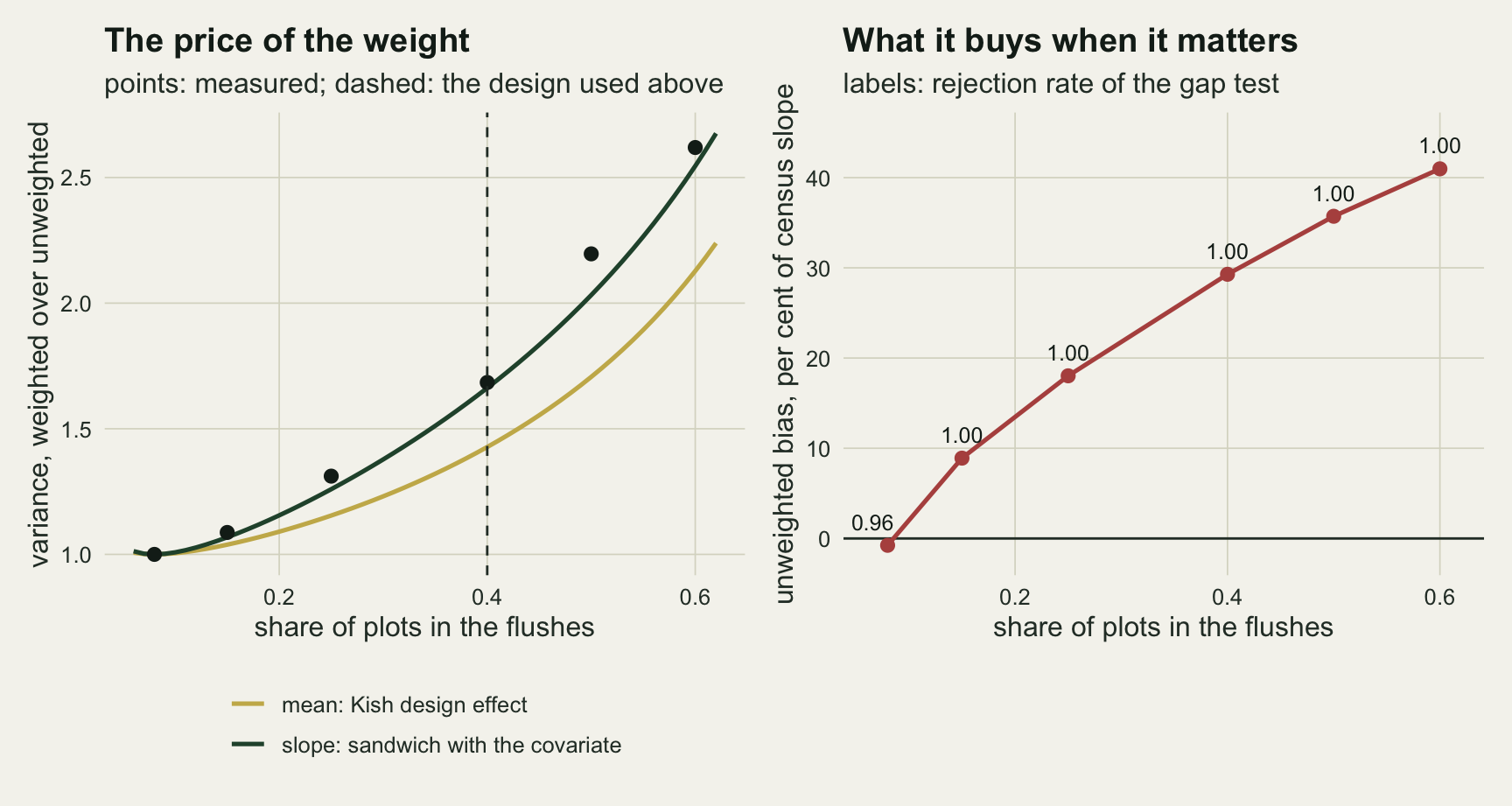
The gap between the fits is the test
If the two fits agree when the model is right and part when it is wrong, their difference is a test of the model. That is DuMouchel and Duncan’s proposal, and here it is the difference of the two slopes divided by the stratified standard error of the difference from the design chunk. Under the three misspecified truths it rejects at the five per cent level in at least 0.986 of samples in every landscape. The harder question is what it does when the model is right, and the answer depends on something a five-landscape run cannot see: every finite landscape departs from its own model a little, so the unweighted fit’s target sits a little off the census slope even when the model is right. The size therefore has to be measured over many landscapes.
# the unweighted fit's own target in a finite landscape
pseudo_u <- function(land, n_r, n_c) {
  in_r <- land$rare == 1L
  x_r <- cbind(1, land$x[in_r]); x_c <- cbind(1, land$x[!in_r])
  a_mat <- n_r * crossprod(x_r) / nrow(x_r) + n_c * crossprod(x_c) / nrow(x_c)
  b_vec <- n_r * crossprod(x_r, land$y[in_r]) / nrow(x_r) +
           n_c * crossprod(x_c, land$y[!in_r]) / nrow(x_c)
  solve(a_mat, b_vec)[2]
}
n_land_null <- 300L
n_rep_null  <- 100L
null_sizes  <- c(300L, 1200L)
set.seed(3104)
null_out <- do.call(rbind, lapply(null_sizes, function(n_all) {
  n_r <- as.integer(0.4 * n_all)
  do.call(rbind, lapply(seq_len(n_land_null), function(k) {
    land  <- make_landscape("right")
    b_pop <- census_slope(land)
    idx_r <- which(land$rare == 1L); idx_c <- which(land$rare == 0L)
    draws <- replicate(n_rep_null, fit_pair(land, idx_r, idx_c, n_r, n_all - n_r))
    data.frame(n_all = n_all, land = k,
               own_gap = 100 * (pseudo_u(land, n_r, n_all - n_r) - b_pop) / b_pop,
               rej_fpc = mean(abs(draws["z_fpc", ]) > z_crit),
               rej_wr  = mean(abs(draws["z_wr", ]) > z_crit),
               sd_z    = sd(draws["z_fpc", ]))
  }))
}))
# landscapes are the independent unit for the Monte Carlo standard error
size_fpc <- tapply(null_out$rej_fpc, null_out$n_all, mean)
size_wr  <- tapply(null_out$rej_wr, null_out$n_all, mean)
se_fpc   <- tapply(null_out$rej_fpc, null_out$n_all, sd) / sqrt(n_land_null)
se_wr    <- tapply(null_out$rej_wr, null_out$n_all, sd) / sqrt(n_land_null)
sd_z_med <- tapply(null_out$sd_z, null_out$n_all, median)
gap_sd   <- sd(null_out$own_gap)
Over 300 landscapes with the model right and 100 samples from each, the test with the finite population correction rejects in 0.0573 of samples at three hundred plots (Monte Carlo standard error 0.0013, with landscapes as the unit) and in 0.0675 at twelve hundred plots (0.0021). It is not a five per cent test. Its variance estimate is not the problem: within a landscape the standard deviation of the test statistic is 1.008 at three hundred plots and 0.997 at twelve hundred (medians over landscapes), as it should be. What moves is the centre. In a finite landscape the best line under the sample’s covariate distribution and the census line differ by chance, by a standard deviation of 1.10 per cent of the census slope over these landscapes, and the design-based test, correctly, sees that difference. It sees it better with more plots, which is why its rejection rate grows with the sample.
Dropping the finite population correction changes the question from this landscape to the model that generated it, and the chance difference is then part of what the variance allows for. That version rejects in 0.0531 of samples at three hundred plots (0.0013) and 0.0492 at twelve hundred (0.0018). Since the question a reader is asking is whether the model is right, the version without the correction is the one used from here on. In the five model-right landscapes of the earlier section the two versions rejected in 0.061 and 0.057 of samples (medians), so on a single survey the choice rarely changes the verdict; it matters for what the verdict means.
gap_grid  <- c(0, 0.1, 0.2, 0.3, 0.45, 0.6)
n_land_sw <- 20L
n_rep_sw  <- 100L
set.seed(3105)
sweep_out <- do.call(rbind, lapply(gap_grid, function(g) {
  per_land <- t(vapply(seq_len(n_land_sw), function(k) {
    land  <- make_landscape("by_strat", gap = g)
    b_pop <- census_slope(land)
    idx_r <- which(land$rare == 1L); idx_c <- which(land$rare == 0L)
    draws <- replicate(n_rep_sw, fit_pair(land, idx_r, idx_c, n_rare, n_plot - n_rare))
    c(pct_u  = 100 * (mean(draws["b_u", ]) - b_pop) / b_pop,
      rej_wr = mean(abs(draws["z_wr", ]) > z_crit))
  }, numeric(2)))
  data.frame(gap = g, pct_u = median(per_land[, "pct_u"]),
             rej_wr = mean(per_land[, "rej_wr"]),
             se_wr  = sd(per_land[, "rej_wr"]) / sqrt(n_land_sw))
}))
pow_at <- function(g) sweep_out$rej_wr[sweep_out$gap == g]
pct_at <- function(g) sweep_out$pct_u[sweep_out$gap == g]
A test is only as useful as the bias it can see. The sweep runs the flush slope from equal to 0.6 steeper, 20 landscapes and 100 samples at each step, with the design above. When the unweighted slope is off by 4.1 per cent of the census slope the test fires in 0.10 of surveys; at 11.3 per cent it fires in 0.48; it needs a bias of about 16 per cent to fire in 0.84. At three hundred plots this is a screen for large departures, not a guarantee that a small bias will be caught.
The allocation sweep in the previous section adds the opposite warning. At proportional allocation the unweighted bias in the steeper-flush landscape is -0.76 per cent, since the sample is then self-weighting, yet the test rejects in 0.96 of samples. With two strata and weights that are constant within a stratum, the gap is, to first order, proportional to the difference between the two weights and so is its standard error, and the ratio keeps testing whether the flushes follow the same line as the slopes however small the weight difference becomes. A rejection says that the model is wrong. How much that matters for the census slope is the size of the gap itself, which is why the gap should be reported with its interval and not as a p value alone.
null_out$plots <- factor(sprintf("%d plots", null_out$n_all),
                         levels = sprintf("%d plots", null_sizes))
p_null <- ggplot(null_out, aes(own_gap, rej_fpc, colour = plots)) +
  geom_hline(yintercept = 0.05, linetype = "dashed", colour = te_body, linewidth = 0.5) +
  geom_point(alpha = 0.5, size = 1.5) +
  scale_colour_manual(values = c(te_gold, te_forest), name = NULL) +
  labs(x = "landscape's own gap, per cent of census slope",
       y = "rejection rate, model right",
       title = "Each landscape has its own null",
       subtitle = "dashed: the nominal five per cent") +
  theme_datasheet() +
  theme(legend.position = "bottom")

p_pow <- ggplot(sweep_out, aes(pct_u, rej_wr)) +
  geom_hline(yintercept = 0.05, linetype = "dashed", colour = te_body, linewidth = 0.5) +
  geom_errorbar(aes(ymin = rej_wr - 1.96 * se_wr, ymax = rej_wr + 1.96 * se_wr),
                width = 0.6, colour = te_rust, linewidth = 0.5) +
  geom_line(colour = te_rust, linewidth = 0.9) +
  geom_point(colour = te_rust, size = 2.3) +
  scale_y_continuous(limits = c(0, 1)) +
  labs(x = "unweighted bias, per cent of census slope",
       y = "rejection rate",
       title = "The screen sees large biases",
       subtitle = "300 plots, 120 in the flushes") +
  theme_datasheet()

(p_null | p_pow) + plot_annotation(theme = theme_datasheet())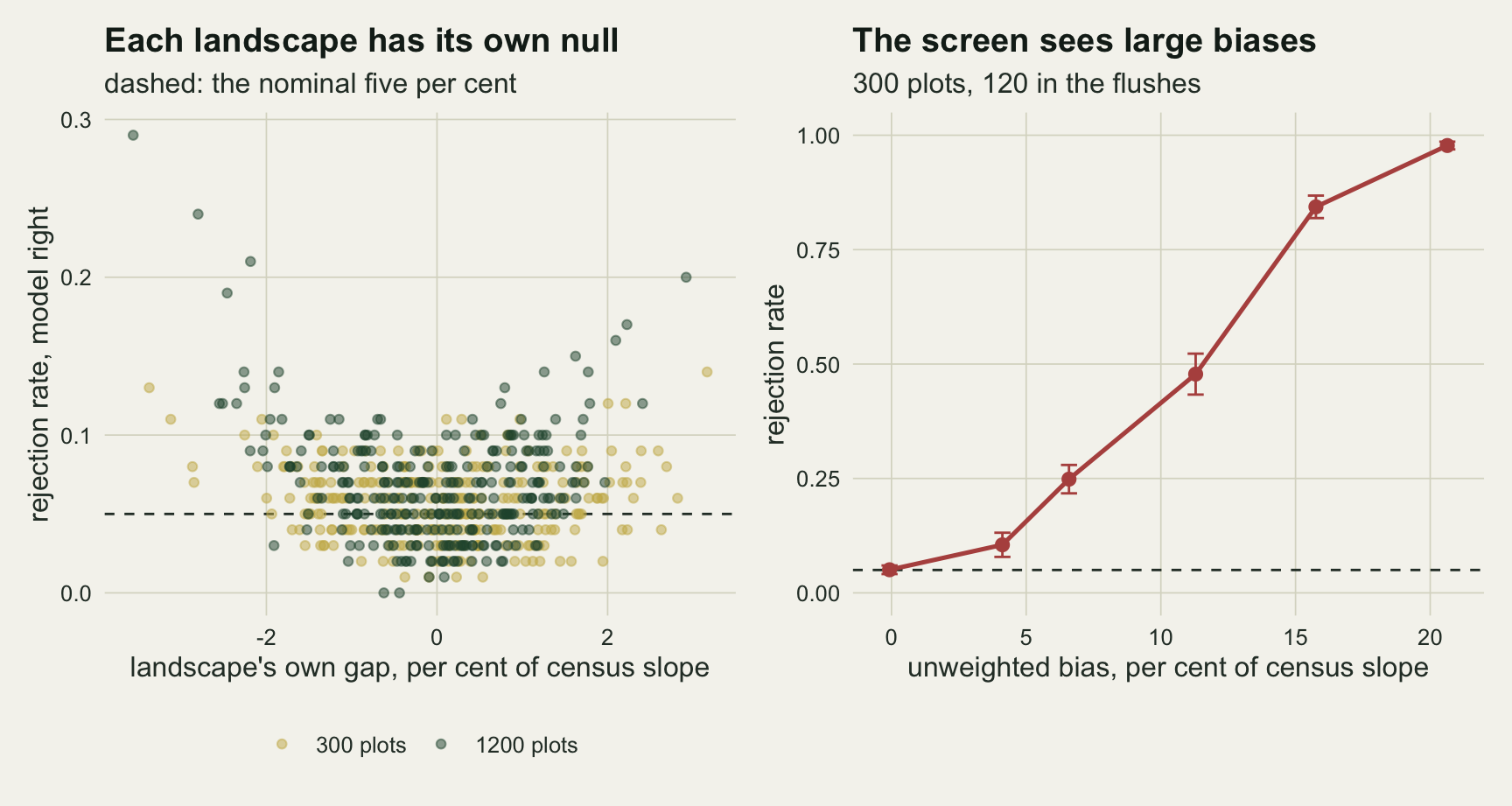
Or fit the stratum and average over the map
A field ecologist reading this may reasonably say that the census slope is the wrong target, and that what the survey found is two slopes, one for the flushes and one for the rest. In that case the answer is to fit the stratum-by-moisture interaction, the weighting question dissolves, and nothing above is needed: within a stratum the sample is a simple random sample, so each stratum’s line is estimated without weights. Pfeffermann’s review makes the general point that putting the design variables into the model is the model-based alternative to weighting.
If the census slope is still wanted, the two stratum lines can be fitted and their predictions averaged over every cell of the map, which needs the moisture index everywhere; a mapped wetness index is the usual source. That is the third estimator carried through the truths chunk. Its bias stays within 0.59 per cent of the census slope under all four truths, including the two curved ones where the stratum lines are themselves wrong. It does not escape the price: with the model right its variance is 1.67 times the unweighted variance, against 1.66 for the weighted fit, and in the steeper-flush landscapes it is 1.42 against 1.45. The census slope costs what it costs because the design put its plots where the census does not.
What to report
Say what the slope is a slope of. A weighted fit estimates the census slope of the surveyed landscape; an unweighted fit estimates the best line for a landscape shaped like the sample, which is the same number only if the model is right. If the question is about the strata themselves, fit the interaction and report the stratum slopes, and the weight is no longer the issue.
Fit both and report both slopes and their difference with a standard error, computed from the stratified linearisation above or from a survey package’s design-based variance. In this design, with the model right, the weighted fit paid about 66 per cent extra variance for nothing, so the unweighted slope is the one to report when the gap is small and its interval is narrow compared with the effect of interest; otherwise report the weighted slope and say that the model failed the check. Choosing the estimator by the test is itself a pre-test procedure, and the interval of whichever slope is reported does not carry that choice.
Do not predict the price from the weights alone. Kish’s design effect of 1.43 came within 4 per cent of the measured price of the mean (1.49) and fell well short of the slope’s measured 1.66; the variance of a coefficient depends on where the strata sit on the covariate, and Kish’s formula also leaves out the finite population correction.
Treat the gap test as a screen. At three hundred plots it caught a bias of about 16 per cent of the slope in 0.84 of surveys and a bias of 4.1 per cent in only 0.10. A non-rejection is not evidence that the unweighted slope is safe to within a few per cent, and a rejection is evidence against the model rather than a measure of the bias.
Honest limits
The design has two strata and one covariate, and the weights are constant within a stratum. With more strata or covariates DuMouchel and Duncan’s test becomes a joint test on several coefficients, usually run as an F test on the weight and its products with the covariates, and its size and power at a few hundred plots were not checked here. Weights that vary within strata, as in probability-proportional-to-size designs, break the link between the gap test and a test of the stratum-by-covariate interaction that showed up at proportional allocation.
The errors are normal with a constant variance in both strata. If the flushes are noisier than the slopes, the unweighted fit is no longer the efficient one, the price changes, and a variance-weighted fit becomes a third candidate that none of the runs here include. The linearised variance used for the test does not assume constant variance, but its behaviour under that departure was not measured.
The test is not exact. Without the finite population correction it rejected in 0.0531 of samples at three hundred plots, a little over the nominal level; with the correction, in 0.0573 at three hundred and 0.0675 at twelve hundred, because it tests the realised landscape and every realised landscape departs a little from its model. Lumley and Scott review design-based inference for regression, including likelihood-ratio and score tests that are alternatives to the Wald form used here; none of those was tried.
The share of plots in the flushes, two in five from a habitat covering eight per cent of the cells, is a strong but ordinary oversampling for a rare target habitat. The allocation sweep shows that both the price and the bias scale with it, and that at proportional allocation there is nothing to decide. The size and power figures are for the design above and change with the allocation.
Plots here are cells drawn at random within strata, with no spatial structure in the noise. Neighbouring plots in a real survey share unmeasured conditions, the effective sample size is smaller than the plot count, and both fits and the test would need a variance that accounts for it.
References
DuMouchel WH, Duncan GJ 1983 Journal of the American Statistical Association 78(383):535-543 (10.1080/01621459.1983.10478006)
Solon G, Haider SJ, Wooldridge JM 2015 Journal of Human Resources 50(2):301-316 (10.3368/jhr.50.2.301)
Pfeffermann D 1993 International Statistical Review 61(2):317-337 (10.2307/1403631)
Lumley T, Scott A 2017 Statistical Science 32(2):265-278 (10.1214/16-STS605)