library(ggplot2)
library(patchwork)

te_paper  <- "#f5f4ee"
te_ink    <- "#16241d"
te_body   <- "#2c3a31"
te_forest <- "#275139"
te_rust   <- "#b5534e"
te_gold   <- "#c9b458"
te_line   <- "#dad9ca"

theme_datasheet <- function() {
  theme_minimal(base_size = 12) +
    theme(plot.background  = element_rect(fill = te_paper, colour = NA),
          panel.background = element_rect(fill = te_paper, colour = NA),
          panel.grid.major = element_line(colour = te_line, linewidth = 0.3),
          panel.grid.minor = element_blank(),
          text             = element_text(colour = te_body),
          plot.title       = element_text(colour = te_ink, face = "bold"),
          plot.subtitle    = element_text(colour = te_body),
          axis.text        = element_text(colour = te_body))
}GPS fix loss and the collars you drop
R
resource selection
movement ecology
telemetry
missing data
simulation
ecology tutorial
Canopy blocks GPS fixes, so the used points in a resource selection function are selected by the habitat under test. Why dropping bad collars is worse, in R.
Forty deer carry GPS collars through a season in mixed forest, and every collar tries for a position 250 times. Where the canopy is open the satellites are in view and almost every attempt returns a fix; under closed canopy a good share of the attempts come back empty. The locations that do come back are joined to a canopy cover layer and go into a resource selection function, the used-available logistic model that asks whether the animals choose cover more often than the forest offers it. Before that, somebody tidies the data. A few collars have delivered far fewer positions than the rest, and the methods section says what methods sections often say in one form or another: animals with too few locations were excluded.
Both steps delete rows, and in both the thing that decides which rows go is canopy, the covariate whose coefficient is being estimated. The first deletion is the fix loss itself, and it is not new. Frair and colleagues showed in 2004 that habitat-dependent fix success biases resource selection models, modelled the fix probability from stationary test collars, and corrected the bias by weighting each location with the inverse of its fix probability, and compared that with an iterative-simulation correction that fills in the missing locations; Frair and colleagues returned to it in 2010 in a wider review of habitat-biased and imprecise GPS locations. The first half of this post is a demonstration of that known result, calibrated so the size of the bias can be read off a line. The second deletion is the subject: a rule stated over collars does its damage on animals, and the weights that repair the points cannot repair it.
The nearest post on this site is coordinate error and habitat assignment. That post makes every location present and slightly wrong, and the damage is attenuation with a formula; here the locations are missing, what makes them missing is the covariate being estimated, and the tidy-up rule that follows selects the animals as well as the points. The estimator is the one built in resource selection functions in R, on complete used points, and everything said there about the coefficient being relative holds here: it is a log ratio of use to availability per unit of canopy and never a probability of anything. The general vocabulary is in missing data: MCAR, MAR and MNAR, which imposes its mechanisms on a measured response and counts complete-case bias. The design here is different in three ways that matter: the response is a used-available contrast whose zeros are drawn by the analyst, the repair run here is a weight estimated from stationary test collars (the simulation correction Frair and colleagues also tested is not run), and there is a second selection stage, on animals, that the generic frame has no place for. That second stage is a case of what collider bias and selection calls selection as conditioning in disguise, and the weighting used below is the same inverse-probability idea as in propensity scores and IPW, applied to observations rather than treatments.
Forty collars, one landscape and a fix model
The landscape is reduced to the one covariate that matters. Canopy cover is recorded in whole per cent, from 0 to 100, and coded as a proportion from 0 to 1, so a coefficient is per change from open to full cover. Every value is equally available to every animal, so availability is matched per animal and nothing below can be a home-range artefact. Each collar has its own selection coefficient, drawn from a normal distribution with mean 1.2 and standard deviation 0.9, and its 250 true positions are drawn with weight exp(beta_i * canopy). Each attempt then returns a fix with probability plogis(3.2 - 3.0 * canopy). Each animal gets 500 available points drawn uniformly over the canopy classes.
All of that is fixed before anything runs. So is the replication: 200 simulated studies of 40 collars for every setting, which is enough to put Monte Carlo standard errors on the quantities that are compared.
canopy   <- seq(0, 1, by = 0.01)
n_cls    <- length(canopy)
n_col    <- 40
n_fix    <- 250
n_avail  <- 500
mu_beta  <- 1.2
sd_beta  <- 0.9
a0_fix   <- 3.2
a1_strong <- -3.0
a1_weak   <- -1.5
n_study  <- 200
thr_grid <- seq(0.55, 0.97, by = 0.01)
thr_rule <- 0.80

q_fix <- function(a1, a0 = a0_fix) plogis(a0 + a1 * canopy)
Because the covariate takes 101 values, a used-available logistic regression can be fitted on counts per canopy class rather than on individual points, and the fit is identical to glm() on the expanded data with case weights. The function below is that fit, written as Newton-Raphson and vectorised over animals so that 40 separate fits cost one matrix operation. Weights enter the used side as non-integer counts, which is how the inverse fix-probability weights are applied later.
fit_rsf <- function(used_w, avail_n, iter = 30) {
  if (is.null(dim(used_w))) {
    used_w  <- matrix(used_w, 1)
    avail_n <- matrix(avail_n, 1)
  }
  n_row <- nrow(used_w)
  x_mat <- matrix(canopy, n_row, n_cls, byrow = TRUE)
  tot   <- used_w + avail_n
  a_hat <- log(rowSums(used_w) / rowSums(avail_n))
  b_hat <- rep(0, n_row)
  for (k in seq_len(iter)) {
    p_hat <- plogis(a_hat + b_hat * x_mat)
    resid <- used_w - tot * p_hat
    g_a <- rowSums(resid)
    g_b <- rowSums(resid * x_mat)
    w_i <- tot * p_hat * (1 - p_hat)
    h_aa <- rowSums(w_i)
    h_ab <- rowSums(w_i * x_mat)
    h_bb <- rowSums(w_i * x_mat^2)
    h_det <- h_aa * h_bb - h_ab^2
    step_b <- (-h_ab * g_a + h_aa * g_b) / h_det
    a_hat <- a_hat + (h_bb * g_a - h_ab * g_b) / h_det
    b_hat <- b_hat + step_b
    if (max(abs(step_b)) < 1e-10) break
  }
  b_hat
}

set.seed(5102)
used_chk  <- rmultinom(1, n_fix, exp(mu_beta * canopy))[, 1]
avail_chk <- rmultinom(1, n_avail, rep(1, n_cls))[, 1]
chk_frame <- data.frame(used = rep(c(1, 0), each = n_cls), cover = rep(canopy, 2),
                        wt = c(used_chk, avail_chk))
glm_slope <- unname(coef(glm(used ~ cover, family = binomial, data = chk_frame,
                             weights = wt))[2])
grid_slope <- fit_rsf(used_chk, avail_chk)
fit_gap <- abs(glm_slope - grid_slope)
On one simulated animal the gridded fit returns 1.063476 and glm() returns 1.063476, a difference of \(6.69 \times 10^{-9}\).
The study simulator draws the true positions, thins them by the fix model, and returns everything the later sections need. Each collar is fitted on its own and on the pooled data of all collars, in three arms: every true position (no loss, which no field study has), the acquired fixes, and the acquired fixes weighted by one over their fix probability. The collar filter is then applied at every threshold in the grid, on the same data.
one_study <- function(a1 = a1_strong, sd_b = sd_beta, keep_data = FALSE) {
  beta_i  <- rnorm(n_col, mu_beta, sd_b)
  q_vec   <- q_fix(a1)
  tilt    <- exp(outer(beta_i, canopy))
  used_n  <- t(apply(tilt, 1, function(w) rmultinom(1, n_fix, w)))
  got_n   <- matrix(rbinom(length(used_n), used_n, rep(q_vec, each = n_col)), n_col)
  avail_n <- t(rmultinom(n_col, n_avail, rep(1, n_cls)))
  got_w   <- sweep(got_n, 2, q_vec, "/")
  success <- rowSums(got_n) / n_fix

  ind_none <- fit_rsf(used_n, avail_n)
  ind_acq  <- fit_rsf(got_n, avail_n)
  ind_ipw  <- fit_rsf(got_w, avail_n)

  filt <- t(vapply(thr_grid, function(th) {
    kept <- success >= th
    if (!any(kept)) return(c(thr = th, n_kept = 0, beta_kept = NA,
                             two_filt = NA, two_filt_ipw = NA,
                             pool_filt = NA, pool_filt_ipw = NA))
    c(thr = th, n_kept = sum(kept), beta_kept = mean(beta_i[kept]),
      two_filt = mean(ind_acq[kept]), two_filt_ipw = mean(ind_ipw[kept]),
      pool_filt = fit_rsf(colSums(got_n[kept, , drop = FALSE]),
                          colSums(avail_n[kept, , drop = FALSE])),
      pool_filt_ipw = fit_rsf(colSums(got_w[kept, , drop = FALSE]),
                              colSums(avail_n[kept, , drop = FALSE])))
  }, numeric(7)))

  out <- list(
    summ = c(truth = mean(beta_i), success = mean(success),
             two_none = mean(ind_none), two_acq = mean(ind_acq), two_ipw = mean(ind_ipw),
             pool_none = fit_rsf(colSums(used_n), colSums(avail_n)),
             pool_acq = fit_rsf(colSums(got_n), colSums(avail_n)),
             pool_ipw = fit_rsf(colSums(got_w), colSums(avail_n))),
    filt = filt,
    collars = data.frame(beta = beta_i, success = success))
  if (keep_data) out$data <- list(got_n = got_n, avail_n = avail_n, beta = beta_i)
  out
}

run_cell <- function(a1, sd_b, keep_data = FALSE) {
  runs <- lapply(seq_len(n_study), function(i) one_study(a1, sd_b, keep_data))
  summ <- as.data.frame(do.call(rbind, lapply(runs, `[[`, "summ")))
  filt <- as.data.frame(do.call(rbind, lapply(seq_along(runs), function(i)
    cbind(study = i, runs[[i]]$filt))))
  filt$truth <- summ$truth[filt$study]
  filt$success <- summ$success[filt$study]
  list(summ = summ, filt = filt, runs = runs)
}
The point-level loss is the known part
Start with the fixes alone, no filter. The acquired positions of one animal are drawn from its true distribution multiplied by the fix probability, so their log density is the animal’s own beta_i * canopy plus log q(canopy). If log q were exactly a straight line in canopy with slope s, the fitted coefficient would be beta_i + s, and the whole bias would be a property of the fix model, knowable before any animal is collared. It is not exactly a straight line, so the least-squares slope of log q over the canopy range is an approximation, and the sweep below checks how good it is across couplings from none to the strong setting used in the rest of the post.
a1_grid <- seq(0, -3, by = -0.5)
n_sweep <- 100
approx_shift <- vapply(a1_grid, function(a1)
  unname(coef(lm(log(q_fix(a1)) ~ canopy))[2]), 0)

set.seed(2004)
sweep_tab <- do.call(rbind, lapply(seq_along(a1_grid), function(j) {
  s_runs <- t(vapply(seq_len(n_sweep), function(i) {
    beta_i  <- rnorm(n_col, mu_beta, sd_beta)
    q_vec   <- q_fix(a1_grid[j])
    used_n  <- t(apply(exp(outer(beta_i, canopy)), 1,
                       function(w) rmultinom(1, n_fix, w)))
    got_n   <- matrix(rbinom(length(used_n), used_n, rep(q_vec, each = n_col)), n_col)
    avail_n <- t(rmultinom(n_col, n_avail, rep(1, n_cls)))
    c(truth = mean(beta_i), success = sum(got_n) / (n_col * n_fix),
      acq = mean(fit_rsf(got_n, avail_n)),
      ipw = mean(fit_rsf(sweep(got_n, 2, q_vec, "/"), avail_n)))
  }, numeric(4)))
  data.frame(a1 = a1_grid[j], success = mean(s_runs[, "success"]),
             acq_bias = mean(s_runs[, "acq"] - s_runs[, "truth"]),
             acq_se = sd(s_runs[, "acq"] - s_runs[, "truth"]) / sqrt(n_sweep),
             ipw_bias = mean(s_runs[, "ipw"] - s_runs[, "truth"]),
             ipw_se = sd(s_runs[, "ipw"] - s_runs[, "truth"]) / sqrt(n_sweep),
             approx = approx_shift[j])
}))
print(round(sweep_tab, 3))
a1 success acq_bias acq_se ipw_bias ipw_se approx
1 0.0 0.961 0.012 0.005 0.012 0.005 0.000
2 -0.5 0.948 -0.014 0.005 0.012 0.005 -0.025
3 -1.0 0.929 -0.063 0.005 0.003 0.005 -0.064
4 -1.5 0.904 -0.126 0.004 0.003 0.004 -0.124
5 -2.0 0.869 -0.221 0.004 0.002 0.004 -0.214
6 -2.5 0.826 -0.349 0.004 0.008 0.004 -0.343
7 -3.0 0.772 -0.532 0.004 0.011 0.005 -0.523strong_row <- sweep_tab[sweep_tab$a1 == a1_strong, ]
weak_row <- sweep_tab[sweep_tab$a1 == a1_weak, ]
approx_err <- max(abs(sweep_tab$acq_bias - sweep_tab$approx))
ipw_worst <- max(abs(sweep_tab$ipw_bias))
ipw_se_max <- max(sweep_tab$ipw_se)The coefficients here are averages of per-animal fits, and the bias is measured against the mean of the 40 true coefficients in the same study, over 100 studies per coupling. At the strong coupling, where the mean fix success is 0.772, the acquired fixes read the coefficient 0.532 too low (Monte Carlo standard error 0.004), and the straight-line approximation predicts 0.523. Across all 7 couplings the approximation misses the measured bias by at most 0.012. At the weak coupling, a mean fix success of 0.904, the bias is -0.126.
Weighting each acquired fix by one over its fix probability removes it. The weighted estimate is never further than 0.012 from the truth at any coupling, with Monte Carlo standard errors of up to 0.005, and a discrepancy of 0.012 (about 2.5 Monte Carlo standard errors) already appears at a coupling of zero, where no fix depends on canopy and every weight is the same, so it is not the weighting. This is the Frair 2004 result, and the reason it works is the Horvitz-Thompson argument: a fix that had a one in two chance of being recorded stands in for two positions, one of which was lost.
sweep_long <- rbind(
  data.frame(a1 = sweep_tab$a1, bias = sweep_tab$acq_bias, arm = "acquired fixes"),
  data.frame(a1 = sweep_tab$a1, bias = sweep_tab$ipw_bias, arm = "acquired fixes, weighted by 1/q"))
ggplot(sweep_long, aes(-a1, bias)) +
  geom_hline(yintercept = 0, colour = te_body, linewidth = 0.4) +
  geom_line(data = sweep_tab, aes(-a1, approx), inherit.aes = FALSE,
            colour = te_rust, linetype = "dashed", linewidth = 0.8) +
  geom_line(aes(colour = arm), linewidth = 0.9) +
  geom_point(aes(colour = arm), size = 2.4) +
  scale_colour_manual(values = c(te_forest, te_gold), name = NULL) +
  labs(x = "strength of canopy effect on fix success (minus a1)",
       y = "bias of the selection coefficient",
       title = "Fix loss shifts the coefficient by the slope of log q",
       subtitle = "dashed red: least-squares slope of log fix probability on canopy") +
  theme_datasheet() +
  theme(legend.position = "bottom")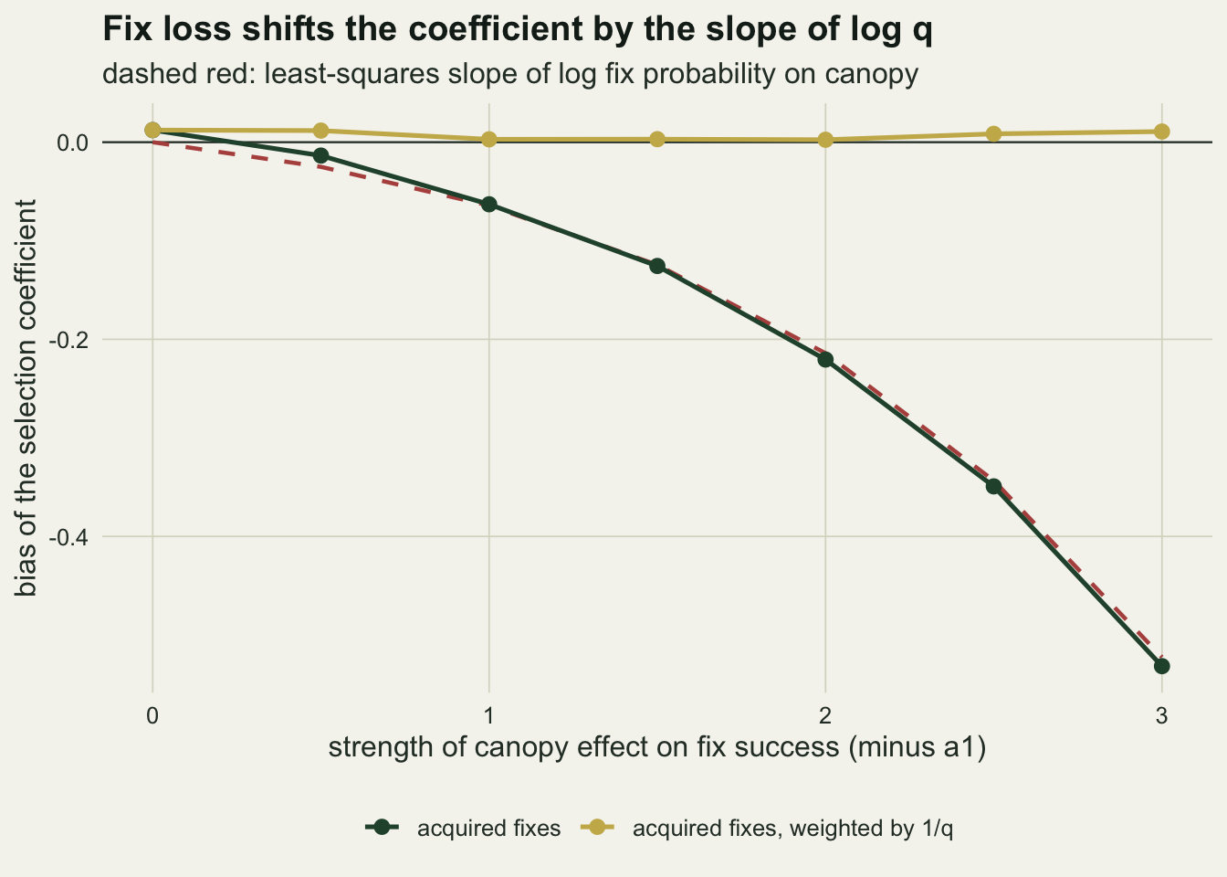
A rule about collars acts on animals
Now the tidy-up. Fix success is counted per collar over its 250 attempted fixes, and the rule keeps a collar when that share is at least 0.80. A rule of “at least 200 locations per animal” is the same rule whenever every collar attempts the same number of fixes, which is why the collar-level version is less exotic than it sounds. Its denominator is collars, not locations, and that mismatch is the point: the rule is stated as a data-quality screen on devices and it acts as a sampling rule on animals.
set.seed(8021)
cell_sh <- run_cell(a1_strong, sd_beta, keep_data = TRUE)
summ_sh <- cell_sh$summ
f_sh    <- cell_sh$filt
at_rule <- f_sh[abs(f_sh$thr - thr_rule) < 1e-9, ]

succ_mean  <- mean(summ_sh$success)
kept_mean  <- mean(at_rule$n_kept)
kept_lo    <- min(at_rule$n_kept)
kept_hi    <- max(at_rule$n_kept)
zero_kept  <- sum(at_rule$n_kept == 0)
gap_rule   <- at_rule$beta_kept - at_rule$truth
gap_mean   <- mean(gap_rule, na.rm = TRUE)
gap_se     <- sd(gap_rule, na.rm = TRUE) / sqrt(sum(!is.na(gap_rule)))
truth_mean <- mean(summ_sh$truth)
kept_beta  <- mean(at_rule$beta_kept, na.rm = TRUE)

coll_all <- do.call(rbind, lapply(cell_sh$runs, `[[`, "collars"))
cor_bs   <- cor(coll_all$beta, coll_all$success)
proxy_cor <- function(r) {
  mean_cov <- as.vector(r$data$got_n %*% canopy) / rowSums(r$data$got_n)
  cor(mean_cov, r$collars$success)
}
prox_sh  <- vapply(cell_sh$runs, proxy_cor, 0)
print(round(c(mean_success = succ_mean, collars_kept = kept_mean,
              truth = truth_mean, beta_kept = kept_beta, gap = gap_mean,
              gap_se = gap_se), 3))
mean_success collars_kept truth beta_kept gap gap_se
0.772 10.370 1.213 0.361 -0.852 0.016 At the strong coupling the mean fix success is 0.772, a little below the threshold, and the rule keeps on average 10.4 of 40 collars (from 2 to 18 across the 200 studies). The collars it keeps are not a random 26 per cent of the animals. Their mean true selection coefficient is 0.361, against a population mean of 1.213: the rule lowers the coefficient of the animals in the analysis by 0.852 (Monte Carlo standard error 0.016) before any model is fitted.
The mechanism is in the figure. A collar’s fix success is high when its animal spent little time under canopy, and an animal spends little time under canopy when its selection coefficient for canopy is low. Across all 8000 simulated collars the correlation between the true coefficient and the realised fix success is -0.75. A threshold on fix success is therefore a threshold on the coefficient being estimated, applied with sampling noise.
coll_show <- do.call(rbind, lapply(1:25, function(i) cell_sh$runs[[i]]$collars))
coll_show$status <- ifelse(coll_show$success >= thr_rule, "kept by the rule", "dropped")
ggplot(coll_show, aes(beta, success, colour = status)) +
  geom_point(size = 1.4, alpha = 0.7) +
  geom_hline(yintercept = thr_rule, linetype = "dashed", colour = te_ink, linewidth = 0.6) +
  geom_vline(xintercept = mu_beta, colour = te_body, linewidth = 0.4) +
  scale_colour_manual(values = c("dropped" = te_line, "kept by the rule" = te_rust),
                      name = NULL) +
  guides(colour = guide_legend(override.aes = list(size = 3, alpha = 1))) +
  labs(x = "true selection coefficient for canopy",
       y = "realised fix success (share of 250 attempts)",
       title = "The collars that pass are the animals that select cover least",
       subtitle = "thin vertical line: the population mean coefficient, 1.2") +
  theme_datasheet() +
  theme(legend.position = "bottom")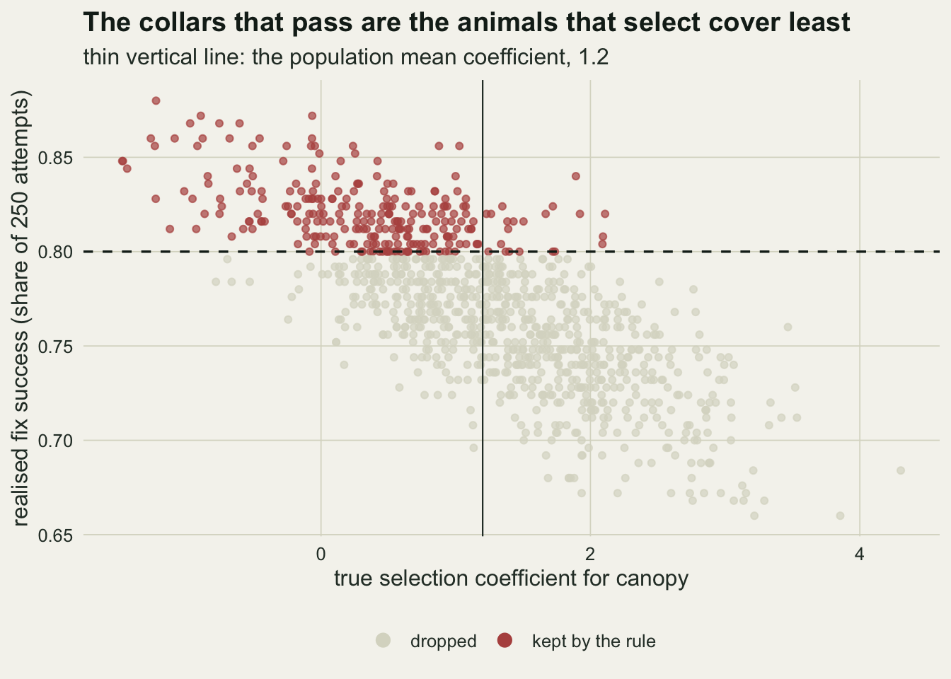
Weighting repairs the points and not the animals
Each arm can now be estimated two ways. The pooled fit puts every retained point of every retained collar into one logistic regression, which is what many analyses do. The two-stage fit estimates each animal separately and averages the coefficients, which treats the animal as the unit of replication, one of the two-stage approaches Fieberg and colleagues review for correlated data in resource selection and suggest as a pragmatic choice. With availability matched per animal, the pooled fit estimates a mixture rather than the mean coefficient, and the no-loss arm shows by how much.
arm_tab <- data.frame(
  arm = c("no loss", "acquired fixes", "acquired, 1/q",
          "collar filter", "collar filter, 1/q"),
  two_stage = c(mean(summ_sh$two_none), mean(summ_sh$two_acq), mean(summ_sh$two_ipw),
                mean(at_rule$two_filt, na.rm = TRUE),
                mean(at_rule$two_filt_ipw, na.rm = TRUE)),
  two_sd = c(sd(summ_sh$two_none), sd(summ_sh$two_acq), sd(summ_sh$two_ipw),
             sd(at_rule$two_filt, na.rm = TRUE), sd(at_rule$two_filt_ipw, na.rm = TRUE)),
  pooled = c(mean(summ_sh$pool_none), mean(summ_sh$pool_acq), mean(summ_sh$pool_ipw),
             mean(at_rule$pool_filt, na.rm = TRUE),
             mean(at_rule$pool_filt_ipw, na.rm = TRUE)))
print(arm_tab, digits = 3)
arm two_stage two_sd pooled
1 no loss 1.213 0.162 1.155
2 acquired fixes 0.667 0.155 0.606
3 acquired, 1/q 1.209 0.160 1.154
4 collar filter -0.165 0.254 -0.168
5 collar filter, 1/q 0.352 0.262 0.354n_valid <- sum(!is.na(at_rule$two_filt))
filt_lo <- quantile(at_rule$two_filt, 0.05, na.rm = TRUE)
filt_hi <- quantile(at_rule$two_filt, 0.95, na.rm = TRUE)
fipw_gap <- at_rule$two_filt_ipw - at_rule$beta_kept
fipw_gap_m <- mean(fipw_gap, na.rm = TRUE)
fipw_gap_se <- sd(fipw_gap, na.rm = TRUE) / sqrt(n_valid)
fipw_bias <- mean(at_rule$two_filt_ipw - at_rule$truth, na.rm = TRUE)
pool_mix <- mean(summ_sh$pool_none - summ_sh$truth)
pool_mix_se <- sd(summ_sh$pool_none - summ_sh$truth) / sqrt(n_study)
two_none_b <- mean(summ_sh$two_none - summ_sh$truth)
two_none_se <- sd(summ_sh$two_none - summ_sh$truth) / sqrt(n_study)
filt_sd_ratio <- arm_tab$two_sd[4] / arm_tab$two_sd[2]
filt_near0 <- mean(abs(at_rule$two_filt) < arm_tab$two_sd[4], na.rm = TRUE)
filt_pos <- mean(at_rule$two_filt > 0, na.rm = TRUE)
filt_max <- max(at_rule$two_filt, na.rm = TRUE)
kept_acq_bias <- mean(at_rule$two_filt - at_rule$beta_kept, na.rm = TRUE)
main_acq_bias <- mean(summ_sh$two_acq - summ_sh$truth)The first three rows repeat the previous section at this coupling. With no loss the two-stage estimate is 1.213 against a mean true coefficient of 1.213 (the paired difference has a standard error of 0.003), while the pooled fit gives 1.155, 0.058 below the mean even with every position present. The acquired fixes give 0.667, and the weights bring that back to 1.209.
After the collar filter the estimate is -0.165 on average, and that average is two damages added together. The kept collars have a mean true coefficient of 0.361, and their acquired fixes read it 0.525 too low, about the same point-level bias as all 40 collars have in these studies (0.546): the selection of animals and the loss of points simply add. Where the sum lands relative to zero depends on the size of each part, which is set by the threshold, the canopy effect and the spread between animals; it says nothing about whether the animals in the study select or avoid cover. The study-to-study standard deviation of the filtered estimate is 0.25, 1.6 times that of the acquired arm, and the middle ninety per cent of studies runs from -0.57 to 0.28. A single study’s estimate lies within one study-to-study standard deviation of zero in 58 per cent of studies, it is above zero in 28 per cent, and the largest of the 200 estimates is 0.59, less than half the population mean of 1.21.
Adding the weights after the filter moves the estimate to 0.352, still 0.861 below the population mean. The two-stage fit shows exactly what the weighted estimate has become: it differs from the mean true coefficient of the retained collars by -0.009 (standard error 0.007). The weights did their job. They recovered the mean selection of the animals in the analysis, and those animals are the ones that select cover least. No per-point weight can put back an animal whose points were all removed, because a weight of one over fix probability only knows how likely a point was to be recorded, not how likely its animal was to survive the screen.
arm_long <- rbind(
  data.frame(arm = "no loss", est = summ_sh$two_none),
  data.frame(arm = "acquired fixes", est = summ_sh$two_acq),
  data.frame(arm = "acquired, 1/q", est = summ_sh$two_ipw),
  data.frame(arm = "collar filter", est = at_rule$two_filt),
  data.frame(arm = "collar filter, 1/q", est = at_rule$two_filt_ipw))
arm_long <- arm_long[!is.na(arm_long$est), ]
arm_long$arm <- factor(arm_long$arm, levels = arm_tab$arm)
arm_long$stage <- ifelse(grepl("filter", arm_long$arm), "after the collar filter",
                         "all collars")
set.seed(71)
ggplot(arm_long, aes(arm, est, colour = stage)) +
  geom_hline(yintercept = truth_mean, linetype = "dashed", colour = te_ink, linewidth = 0.6) +
  geom_hline(yintercept = kept_beta, linetype = "dotted", colour = te_rust, linewidth = 0.8) +
  geom_hline(yintercept = 0, colour = te_body, linewidth = 0.3) +
  geom_jitter(width = 0.18, height = 0, size = 1.1, alpha = 0.45) +
  stat_summary(fun = mean, geom = "point", shape = 23, size = 3.4,
               fill = te_ink, colour = te_paper) +
  scale_colour_manual(values = c("all collars" = te_forest,
                                 "after the collar filter" = te_rust), name = NULL) +
  guides(colour = guide_legend(override.aes = list(size = 3, alpha = 1))) +
  labs(x = NULL, y = "averaged per-animal coefficient",
       title = "The weights fix the points; the filter changed the animals",
       subtitle = "diamonds: means over studies") +
  theme_datasheet() +
  theme(legend.position = "bottom")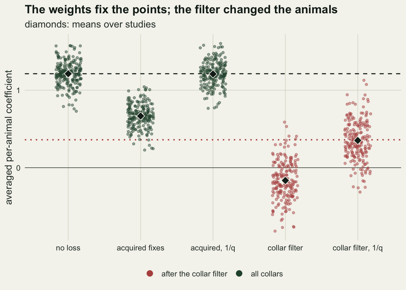
When every animal selects alike, the filter is harmless
The claim so far is that the filter does its damage through variation between animals. That can be tested directly by switching the variation off: the same fix model and the same rule, with every animal given the coefficient 1.2.
set.seed(8022)
cell_sm <- run_cell(a1_strong, 0, keep_data = TRUE)
at_hom  <- cell_sm$filt[abs(cell_sm$filt$thr - thr_rule) < 1e-9, ]
hom_kept    <- mean(at_hom$n_kept)
hom_zero    <- sum(at_hom$n_kept == 0)
hom_acq     <- mean(cell_sm$summ$two_acq)
hom_filt    <- mean(at_hom$two_filt, na.rm = TRUE)
hom_fipw    <- mean(at_hom$two_filt_ipw, na.rm = TRUE)
hom_diff    <- at_hom$two_filt - cell_sm$summ$two_acq[at_hom$study]
hom_diff_m  <- mean(hom_diff, na.rm = TRUE)
hom_diff_se <- sd(hom_diff, na.rm = TRUE) / sqrt(sum(!is.na(hom_diff)))
het_diff    <- at_rule$two_filt - summ_sh$two_acq[at_rule$study]
het_diff_m  <- mean(het_diff, na.rm = TRUE)
prox_sm     <- vapply(cell_sm$runs, proxy_cor, 0)
print(round(c(kept = hom_kept, zero = hom_zero, acquired = hom_acq, filtered = hom_filt,
              filtered_ipw = hom_fipw, diff = hom_diff_m, diff_se = hom_diff_se), 3))
kept zero acquired filtered filtered_ipw diff
6.530 0.000 0.665 0.659 1.199 -0.006
diff_se
0.008 With identical animals the rule keeps fewer collars, 6.5 of 40 on average, because now only sampling luck separates them, and it keeps at least one collar in 200 of 200 studies. But the collars it keeps are exchangeable with the ones it drops. The filtered estimate is 0.659 against 0.665 for all acquired fixes, a paired difference of -0.006 (standard error 0.008), against -0.831 when the animals differ. Filter plus weights returns 1.199 for a true value of 1.2. As a share of the heterogeneous damage that is indistinguishable from zero: the paired difference is within one standard error of it. The damage is selection on the individual coefficient, and without individual differences there is nothing for the rule to select on.
A cliff at the mean fix success
A single threshold of 0.80 is not a finding a reader can carry to their own collars. What matters is where the threshold sits relative to the fix success the collars actually achieve, so the sweep below runs the rule from 0.55 to 0.97 in steps of 0.01 on all four combinations of strong or weak coupling and variable or identical animals, and plots the change the rule makes to the estimate (filtered minus unfiltered, from the same studies) against the threshold minus the mean fix success of the study. The table columns are the threshold, that distance, the share of collars kept, the share of studies left with none, the kept-collar gap in true coefficients and the change in the estimate.
set.seed(8023)
cell_wh <- run_cell(a1_weak, sd_beta)
set.seed(8024)
cell_wm <- run_cell(a1_weak, 0)

sweep_of <- function(cell, lab) {
  ff <- cell$filt
  ff$gap <- ff$beta_kept - ff$truth
  ff$dmg <- ff$two_filt - cell$summ$two_acq[ff$study]
  ff$dist <- ff$thr - ff$success
  out <- do.call(rbind, lapply(split(ff, ff$thr), function(z) data.frame(
    thr = z$thr[1], dist = mean(z$dist), share_kept = mean(z$n_kept) / n_col,
    zero_share = mean(z$n_kept == 0), gap = mean(z$gap, na.rm = TRUE),
    gap_se = sd(z$gap, na.rm = TRUE) / sqrt(sum(!is.na(z$gap))),
    dmg = mean(z$dmg, na.rm = TRUE))))
  rownames(out) <- NULL
  out$setting <- lab
  out
}
cliff <- rbind(sweep_of(cell_sh, "strong coupling, animals differ"),
               sweep_of(cell_sm, "strong coupling, animals alike"),
               sweep_of(cell_wh, "weak coupling, animals differ"),
               sweep_of(cell_wm, "weak coupling, animals alike"))
cliff$setting <- factor(cliff$setting, levels = unique(cliff$setting))

sh_c <- cliff[cliff$setting == "strong coupling, animals differ", ]
row_at <- function(tab, th) tab[abs(tab$thr - th) < 1e-9, ]
sh_60 <- row_at(sh_c, 0.60); sh_70 <- row_at(sh_c, 0.70)
sh_75 <- row_at(sh_c, 0.75); sh_80 <- row_at(sh_c, 0.80); sh_85 <- row_at(sh_c, 0.85)
sh_90 <- row_at(sh_c, 0.90)
wh_c  <- cliff[cliff$setting == "weak coupling, animals differ", ]
succ_weak <- mean(cell_wh$summ$success)
wh_85 <- row_at(wh_c, 0.85); wh_90 <- row_at(wh_c, 0.90)
wh_92 <- row_at(wh_c, 0.92); wh_94 <- row_at(wh_c, 0.94)
wh_acq_bias <- mean(cell_wh$summ$two_acq - cell_wh$summ$truth)
show_cols <- c("thr", "dist", "share_kept", "zero_share", "gap", "dmg")
print(round(sh_c[round(sh_c$thr, 2) %in% c(0.6, 0.7, 0.75, 0.8, 0.85, 0.9), show_cols], 3),
      row.names = FALSE)
thr dist share_kept zero_share gap dmg
0.60 -0.172 1.000 0.000 0.000 0.000
0.70 -0.072 0.962 0.000 -0.053 -0.051
0.75 -0.022 0.712 0.000 -0.318 -0.307
0.80 0.028 0.259 0.000 -0.852 -0.831
0.85 0.078 0.024 0.385 -1.642 -1.597
0.90 0.128 0.000 0.980 -2.723 -2.499print(round(wh_c[round(wh_c$thr, 2) %in% c(0.8, 0.85, 0.9, 0.92, 0.94, 0.96), show_cols], 3),
row.names = FALSE) thr dist share_kept zero_share gap dmg
0.80 -0.103 1.000 0.000 0.000 0.000
0.85 -0.053 0.992 0.000 -0.009 -0.009
0.90 -0.003 0.533 0.000 -0.284 -0.283
0.92 0.017 0.235 0.000 -0.491 -0.483
0.94 0.037 0.021 0.435 -0.848 -0.820
0.96 0.057 0.001 0.965 -1.402 -1.292alike_c <- cliff[cliff$setting == "strong coupling, animals alike" & cliff$zero_share <= 0.10, ]
alike_lo <- min(alike_c$dmg); alike_hi <- max(alike_c$dmg)Under strong coupling with variable animals the rule does little while the threshold sits well below the mean success. At 0.60 it keeps 100.0 per cent of collars and at 0.70 96.2 per cent, and the mean true coefficient of the kept collars is 0.053 below the population mean at 0.70. At 0.75, 0.02 below the mean success, the gap is 0.318; at 0.80, 0.03 above it, the gap is 0.852. At 0.85 the rule keeps 2.4 per cent of collars and returns no collar at all in 38 per cent of studies, and at 0.90 it empties 98 per cent of them. The usable range of the rule and the damaging range of the rule are the same few hundredths either side of the mean fix success.
Weak coupling shifts the whole picture, and a reader whose collars average above 0.90 should take this paragraph as theirs. In the 200 weak-coupling studies the mean fix success is 0.903, the acquired fixes are biased by -0.122, and at 0.85 the rule keeps 99.2 per cent of collars, and those are 0.009 below the population mean. But the same cliff arrives when the threshold reaches the mean: at 0.92, 0.017 above the mean success, the kept collars are 0.491 below the population mean, and at 0.94 the rule empties 44 per cent of studies. Collars with high average success are not protected from the rule; they are protected by a threshold set well below their average.
The figure shows what reaches the estimate. With variable animals the change it plots is the kept-collar gap plus a small difference in point-level bias, and at 0.80 under strong coupling it is -0.831. With animals alike it stays between -0.006 and +0.020 over the plotted strong-coupling range: with nothing to select on, the filter barely moves the estimate.
cliff_show <- cliff[cliff$zero_share <= 0.10, ]
set_cols <- c("strong coupling, animals differ" = te_rust,
              "strong coupling, animals alike" = te_gold,
              "weak coupling, animals differ" = te_forest,
              "weak coupling, animals alike" = te_ink)
p_gap <- ggplot(cliff_show, aes(dist, dmg, colour = setting)) +
  geom_vline(xintercept = 0, linetype = "dashed", colour = te_body, linewidth = 0.4) +
  geom_hline(yintercept = 0, colour = te_body, linewidth = 0.3) +
  geom_line(linewidth = 0.9) +
  scale_colour_manual(values = set_cols, name = NULL) +
  labs(x = "threshold minus mean fix success", y = "filtered minus unfiltered estimate",
       title = "Change in the estimate") +
  theme_datasheet()
p_kept <- ggplot(cliff_show, aes(dist, share_kept, colour = setting)) +
  geom_vline(xintercept = 0, linetype = "dashed", colour = te_body, linewidth = 0.4) +
  geom_line(linewidth = 0.9) +
  scale_colour_manual(values = set_cols, name = NULL) +
  scale_y_continuous(limits = c(0, 1)) +
  labs(x = "threshold minus mean fix success", y = "share of collars kept",
       title = "Collars kept") +
  theme_datasheet()
(p_gap | p_kept) +
  plot_layout(guides = "collect") +
  plot_annotation(theme = theme_datasheet()) &
  theme(legend.position = "bottom") &
  guides(colour = guide_legend(nrow = 2))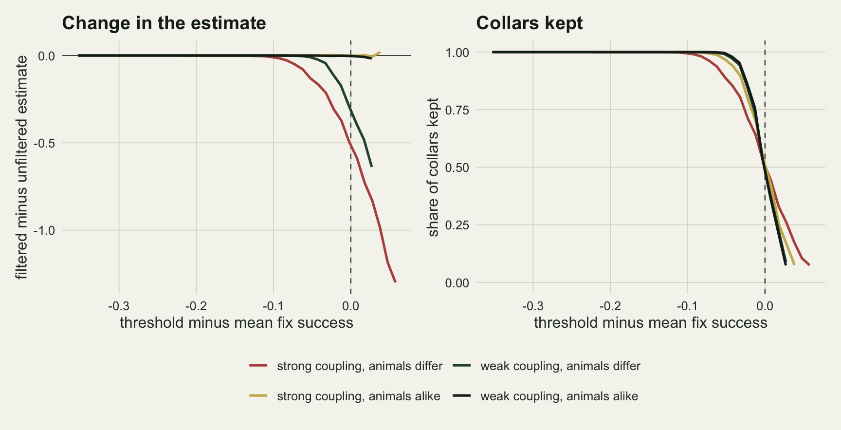
When q has to be estimated
The repair used so far had the true fix probability. A field team does not. It places stationary test collars at sites of known canopy, counts how many attempts return a fix, and fits a logistic regression of fix success on canopy. Two realistic test designs are run here on the strong-coupling studies, each with a fresh set of test collars per study: ten test sites spread across the whole canopy range, and ten sites restricted to canopy of 40 per cent or less, which is where test collars can end up when they have to be put out and collected on foot. Each test site records 100 attempts.
A test design only matters through the shape of the estimated fix model, so the same studies are also reweighted with a fix model whose canopy slope is the true slope multiplied by a factor from 0 (no weighting at all) to 2.5 (weights far too steep). That sweep answers the question of how wrong q can be before the weighting does more harm than leaving it out.
n_test   <- 10
m_test   <- 100
test_all  <- seq(0.05, 0.95, length.out = n_test)
test_open <- seq(0, 0.40, length.out = n_test)
q_true <- q_fix(a1_strong)

est_q <- function(sites) {
  hits <- rbinom(n_test, m_test, plogis(a0_fix + a1_strong * sites))
  cf <- coef(glm(cbind(hits, m_test - hits) ~ sites, family = binomial))
  list(q_hat = plogis(cf[1] + cf[2] * canopy), ratio = unname(cf[2] / a1_strong))
}

set.seed(9031)
test_res <- t(vapply(cell_sh$runs, function(r) {
  dd <- r$data
  qa <- est_q(test_all)
  qo <- est_q(test_open)
  c(truth = mean(dd$beta),
    known = mean(fit_rsf(sweep(dd$got_n, 2, q_true, "/"), dd$avail_n)),
    all_sites = mean(fit_rsf(sweep(dd$got_n, 2, qa$q_hat, "/"), dd$avail_n)),
    open_sites = mean(fit_rsf(sweep(dd$got_n, 2, qo$q_hat, "/"), dd$avail_n)),
    none = mean(fit_rsf(dd$got_n, dd$avail_n)),
    ratio_all = qa$ratio, ratio_open = qo$ratio)
}, numeric(7)))
test_res <- as.data.frame(test_res)

k_grid <- seq(0, 2.5, by = 0.25)
k_bias <- vapply(k_grid, function(k) {
  q_k <- q_fix(k * a1_strong)
  mean(vapply(cell_sh$runs, function(r)
    mean(fit_rsf(sweep(r$data$got_n, 2, q_k, "/"), r$data$avail_n)) - mean(r$data$beta), 0))
}, 0)
k_tab <- data.frame(k = k_grid, bias = k_bias)
none_bias <- k_bias[1]
k_break <- approx(k_tab$bias[k_grid >= 1], k_grid[k_grid >= 1], xout = -none_bias)$y

bias_of <- function(v) c(mean = mean(v - test_res$truth), sd = sd(v - test_res$truth),
                         p90 = unname(quantile(abs(v - test_res$truth), 0.90)))
b_known <- bias_of(test_res$known)
b_all   <- bias_of(test_res$all_sites)
b_open  <- bias_of(test_res$open_sites)
b_none  <- bias_of(test_res$none)
r_all   <- quantile(test_res$ratio_all, c(0.05, 0.95))
r_open  <- quantile(test_res$ratio_open, c(0.05, 0.95))
open_over <- mean(test_res$ratio_open > k_break)
worse_open <- mean(abs(test_res$open_sites - test_res$truth) >
                   abs(test_res$none - test_res$truth))
worse_all  <- mean(abs(test_res$all_sites - test_res$truth) >
                   abs(test_res$none - test_res$truth))
print(round(rbind(known = b_known, all_sites = b_all, open_sites = b_open, none = b_none), 3))
mean sd p90
known -0.004 0.047 0.075
all_sites -0.008 0.076 0.121
open_sites 0.110 0.397 0.706
none -0.546 0.046 0.605print(round(k_tab, 3)) k bias
1 0.00 -0.546
2 0.25 -0.504
3 0.50 -0.422
4 0.75 -0.269
5 1.00 -0.004
6 1.25 0.416
7 1.50 1.010
8 1.75 1.759
9 2.00 2.618
10 2.25 3.536
11 2.50 4.480Weighting by a fix model whose slope is too shallow corrects only part of the bias, and one whose slope is too steep overshoots, so the bias passes through zero near the true slope. Unweighted, the bias in these 200 strong-coupling studies is -0.546; the overcorrection reaches the same size with the opposite sign when the slope of the fix model is 1.30 times the true one. Anything between no weighting and that factor is an improvement on doing nothing.
The test collars decide where a real study lands on that line. With sites spread over the whole canopy range, the estimated slope is between 0.83 and 1.22 times the true slope in ninety per cent of studies, and the weighted estimate has a mean bias of -0.008 with a study-to-study standard deviation of 0.076, against -0.004 and 0.047 with the true q. The weighted estimate is further from the truth than the unweighted one in 0 of the 200 studies. With the sites confined to open canopy, the fix model has to be extrapolated to the closed canopy where fix loss is heaviest: the slope ratio spreads from 0.48 to 1.59, it passes the break-even factor in 20.5 per cent of studies, the weighted estimate has a standard deviation of 0.397, and it is further from the truth than no weighting in 15.0 per cent of studies.
p_k <- ggplot(k_tab, aes(k, bias)) +
  annotate("rect", xmin = -Inf, xmax = Inf, ymin = none_bias, ymax = -none_bias,
           fill = te_line, alpha = 0.5) +
  geom_hline(yintercept = 0, colour = te_body, linewidth = 0.3) +
  geom_vline(xintercept = 1, linetype = "dashed", colour = te_body, linewidth = 0.4) +
  geom_line(colour = te_forest, linewidth = 0.9) +
  geom_point(colour = te_forest, size = 2.2) +
  labs(x = "fix-model slope / true slope", y = "bias of weighted estimate",
       title = "How wrong q can be",
       subtitle = "grey band: smaller bias than no weighting") +
  theme_datasheet()
q_long <- rbind(
  data.frame(arm = "true q", bias = test_res$known - test_res$truth),
  data.frame(arm = "test sites, full range", bias = test_res$all_sites - test_res$truth),
  data.frame(arm = "test sites, open only", bias = test_res$open_sites - test_res$truth),
  data.frame(arm = "no weights", bias = test_res$none - test_res$truth))
q_long$arm <- factor(q_long$arm, levels = unique(q_long$arm))
set.seed(72)
p_q <- ggplot(q_long, aes(arm, bias)) +
  geom_hline(yintercept = 0, colour = te_body, linewidth = 0.3) +
  geom_jitter(width = 0.18, height = 0, size = 1, alpha = 0.45, colour = te_rust) +
  stat_summary(fun = mean, geom = "point", shape = 23, size = 3.2,
               fill = te_ink, colour = te_paper) +
  scale_x_discrete(labels = c("true q", "tests,\nfull range", "tests,\nopen only",
                              "no\nweights")) +
  labs(x = NULL, y = "bias per study", title = "Estimated from test collars") +
  theme_datasheet()
(p_k | p_q) + plot_annotation(theme = theme_datasheet())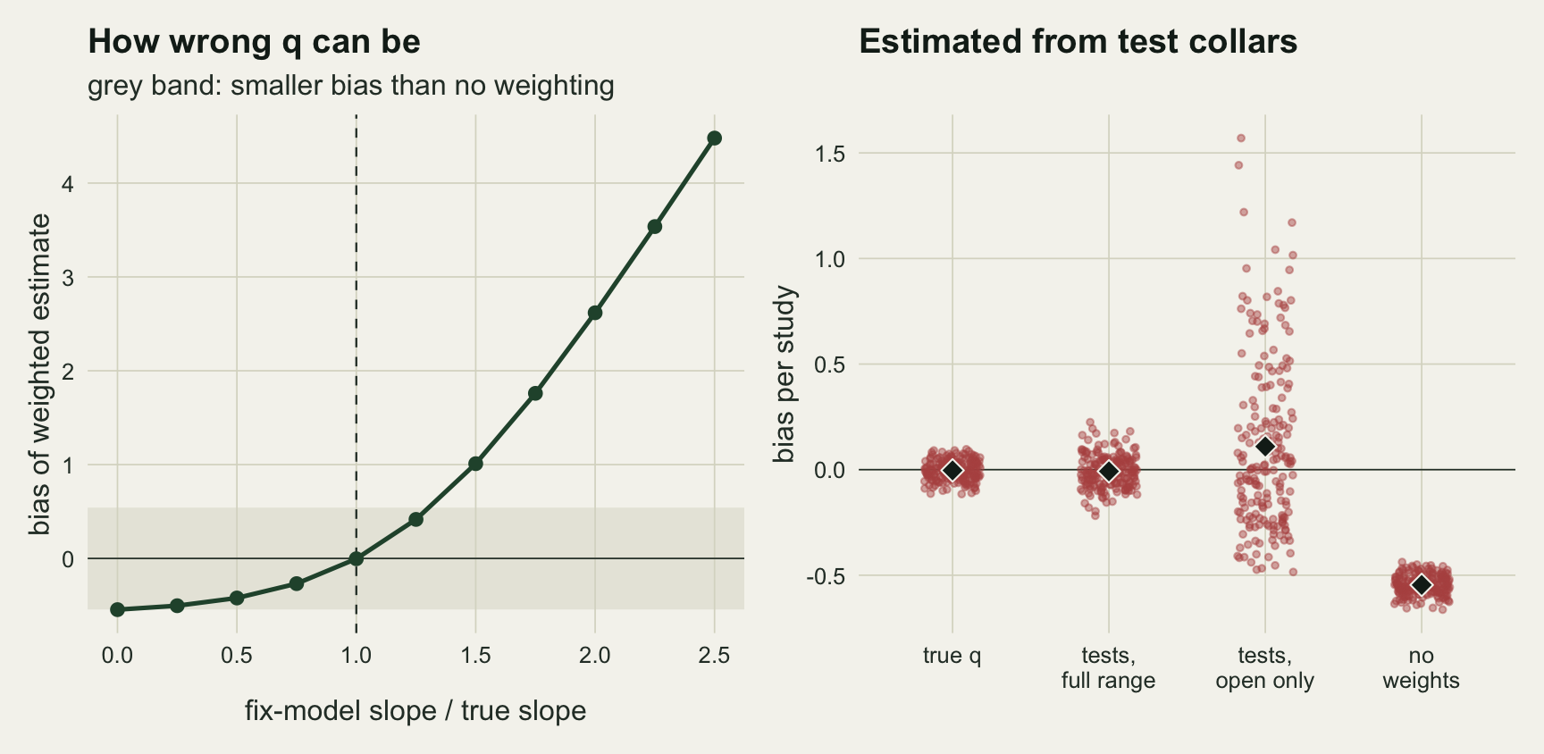
The pooled interval counts fixes, not animals
The sections so far measure bias. The interval around the estimate has a problem of its own: the positions above were drawn independently, and a collar with a short fix interval does not record them that way, because an animal bedded under cover at one fix is likely to be under cover at the next. The pooled fit counts every fix as a separate piece of evidence. Half of the consequence is measured in step selection functions, whose pooling section shows that when animals differ the pooled standard error misses a cluster design effect, DE = 1 + sigma^2 * S * Vw, and whose steps are independent by construction. This section adds the other half, serial dependence along a track, on this post’s design with no fix loss (the no-loss arm), so that only the order of the positions changes.
Each track is a latent autoregressive Gaussian series with lag-one correlation rho, turned into canopy classes through the inverse of the animal’s own distribution exp(beta_i * canopy), so every position keeps the distribution the simulator above draws from and rho 0 is its independent draw. Each collar still records 250 positions: a larger rho stands for fixes taken closer together, not for more of them, which keeps thinning (fewer fixes and less autocorrelation at once) out of the comparison. Three 95 per cent intervals are compared: the pooled Wald interval for the population mean of 1.2, with the standard error from the Newton system of fit_rsf(); each animal’s own Wald interval for its own coefficient; and a two-stage t interval with 39 degrees of freedom on the 40 per-animal slopes. The six cells (rho 0, 0.8 and 0.95, animals alike or differing as before) were fixed before anything was run; a first run had 200 studies per cell, and the table has 400.
se_rsf <- function(used_w, avail_n, b_hat, iter = 30) {
  if (is.null(dim(used_w))) { used_w <- matrix(used_w, 1); avail_n <- matrix(avail_n, 1) }
  x_mat <- matrix(canopy, nrow(used_w), n_cls, byrow = TRUE)
  tot   <- used_w + avail_n
  a_hat <- log(rowSums(used_w) / rowSums(exp(b_hat * x_mat) * avail_n))
  for (k in seq_len(iter)) {  # Newton on the intercept at the fitted slope
    p_hat <- plogis(a_hat + b_hat * x_mat); w_i <- tot * p_hat * (1 - p_hat)
    a_step <- rowSums(used_w - tot * p_hat) / rowSums(w_i); a_hat <- a_hat + a_step
    if (max(abs(a_step)) < 1e-12) break
  }
  sqrt(rowSums(w_i) / (rowSums(w_i) * rowSums(w_i * x_mat^2) - rowSums(w_i * x_mat)^2))
}
# tightened tolerance: glm's default stops its standard error slightly short of convergence
glm_se <- summary(glm(used ~ cover, family = binomial, data = chk_frame, weights = wt,
                      control = glm.control(epsilon = 1e-10)))$coefficients[2, 2]
stopifnot(isTRUE(all.equal(se_rsf(used_chk, avail_chk, grid_slope), glm_se, tolerance = 1e-6)))
track_classes <- function(beta_i, rho, n_pos = n_fix) {
  z_mat <- matrix(rnorm(length(beta_i) * n_pos), length(beta_i), n_pos)
  for (j in 2:n_pos) z_mat[, j] <- rho * z_mat[, j - 1] + sqrt(1 - rho^2) * z_mat[, j]
  t(vapply(seq_along(beta_i), function(i) {
    cdf <- cumsum(exp(beta_i[i] * canopy)); findInterval(pnorm(z_mat[i, ]), cdf / cdf[n_cls]) + 1
  }, numeric(n_pos)))
}
ac_study <- function(rho, sd_b, z95 = qnorm(0.975)) {
  beta_i  <- rnorm(n_col, mu_beta, sd_b)
  used_n  <- t(apply(track_classes(beta_i, rho), 1, tabulate, nbins = n_cls))
  avail_n <- t(rmultinom(n_col, n_avail, rep(1, n_cls)))
  b_pool  <- fit_rsf(colSums(used_n), colSums(avail_n))
  s_pool  <- se_rsf(colSums(used_n), colSums(avail_n), b_pool)
  b_ind   <- fit_rsf(used_n, avail_n)
  t_half  <- qt(0.975, n_col - 1) * sd(b_ind) / sqrt(n_col)
  c(pooled = abs(b_pool - mu_beta) < z95 * s_pool,
    single = mean(abs(b_ind - beta_i) < z95 * se_rsf(used_n, avail_n, b_ind)),
    two_stage = abs(mean(b_ind) - mu_beta) < t_half, two_hi = mean(b_ind) - t_half > mu_beta,
    two_lo = mean(b_ind) + t_half < mu_beta, ind_bias = mean(b_ind - beta_i),
    b_pool = b_pool, s_pool = s_pool)
}
ac_cell <- function(rho, sd_b, z95 = qnorm(0.975)) {
  r_mat <- replicate(ac_reps, ac_study(rho, sd_b))
  est <- r_mat["b_pool", ]; s_rep <- mean(r_mat["s_pool", ]); p_bias <- mean(est) - mu_beta
  # coverage of a normal estimator with this bias, this spread and this reported SE
  c(sd_b = sd_b, rho = rho, rowMeans(r_mat[c("pooled", "single", "two_stage", "two_hi",
                                              "two_lo", "ind_bias"), ]),
    spread = sd(est) / s_rep, normal = pnorm((z95 * s_rep - p_bias) / sd(est)) -
      pnorm((-z95 * s_rep - p_bias) / sd(est)))
}
ac_rho <- c(0, 0.8, 0.95); ac_reps <- 400
set.seed(3451)
ac_tab <- as.data.frame(t(mapply(ac_cell, rep(ac_rho, 2), rep(c(0, sd_beta), each = 3))))
set.seed(3452)
ac_lag <- vapply(ac_rho, function(rho) {
  cc <- canopy[track_classes(mu_beta, rho, 20000)[1, ]]; cor(cc[-1], cc[-20000]) }, 0)
# ac_F: variance of a 250-fix track's mean canopy against independent fixes;
# ac_s: the used side's share of the slope's sampling variance (variance / number of points)
ac_F <- vapply(ac_rho, function(rho)
  var(rowMeans(matrix(canopy[track_classes(rep(mu_beta, 4000), rho)], 4000))), 0)
ac_F <- ac_F / ac_F[1]
p_use <- exp(mu_beta * canopy) / sum(exp(mu_beta * canopy))
v_use <- sum(p_use * (canopy - sum(p_use * canopy))^2) / n_fix
ac_s  <- v_use / (v_use + mean((canopy - mean(canopy))^2) / n_avail)
ac_pred <- sqrt(ac_s * ac_F + 1 - ac_s)
ac_tab$lag1 <- rep(ac_lag, 2); ac_mcse <- sqrt(0.95 * 0.05 / ac_reps)
ac_alike <- ac_tab[ac_tab$sd_b == 0, ]; ac_diff <- ac_tab[ac_tab$sd_b > 0, ]
stopifnot(all(abs(ac_pred[-1] / ac_alike$spread[-1] - 1) < 0.15),
          all(ac_alike$two_hi[3] > ac_alike$two_lo[3], ac_diff$two_hi[3] > ac_diff$two_lo[3]))
print(round(ac_tab[, c("sd_b", "lag1", "pooled", "single", "two_stage", "two_hi", "two_lo",
                       "spread", "normal", "ind_bias")], 3), row.names = FALSE)
sd_b lag1 pooled single two_stage two_hi two_lo spread normal ind_bias
0.0 0.000 0.963 0.952 0.958 0.025 0.018 0.992 0.952 0.006
0.0 0.789 0.610 0.581 0.970 0.015 0.015 2.253 0.609 0.016
0.0 0.946 0.312 0.305 0.930 0.068 0.002 4.873 0.312 0.161
0.9 0.000 0.410 0.949 0.960 0.013 0.028 3.285 0.417 0.003
0.9 0.789 0.340 0.577 0.953 0.035 0.013 4.017 0.357 0.029
0.9 0.946 0.255 0.301 0.930 0.062 0.007 5.783 0.254 0.130print(round(rbind(track_mean = sqrt(ac_F), expected = ac_pred, measured = ac_alike$spread), 2)) [,1] [,2] [,3]
track_mean 1.00 2.91 5.93
expected 1.00 2.42 4.82
measured 0.99 2.25 4.87With identical animals and independent fixes all three intervals hold their level: the pooled interval covers 1.2 in 0.963 of studies, the single-animal interval covers each animal’s own coefficient in 0.952 of animal fits, and the two-stage interval covers in 0.958 (Monte Carlo standard error about 0.011 at 0.95). At rho 0.8, a lag-one autocorrelation of canopy of 0.79 along a long track, the pooled interval covers 0.610, and at rho 0.95 (lag-one 0.95) it covers 0.312. The single-animal interval fails the same way, 0.581 and 0.305, so fitting the animals one at a time does not help while each fit trusts its own Wald standard error. The pooled estimate varies from study to study 2.3 and 4.9 times as much as its reported standard error says, and a normal estimator with that ratio and the measured bias would cover within 0.017 of the simulated rate in every cell: the coverage is what the too-small standard error predicts. For the mean of an autoregressive series with the same lag-one values the factor would be sqrt((1 + r) / (1 - r)), 2.9 and 6.0 (see temporal autocorrelation and effective sample size), and the mean canopy of a 250-fix track here is 2.9 and 5.9 times as variable as with independent fixes: the used positions carry that inflation almost in full. The available points do not. They are independent, and they carry about a third of the slope’s sampling variance (the used share s, from the variance of canopy over the number of points on each side, is 0.65), so with F the square of the track factor the expected factor is sqrt(s * F + 1 - s), 2.4 and 4.8, against the measured 2.3 and 4.9. The share is an approximation from the two means, not the exact variance of a logistic slope.
When the animals differ the pooled interval covers only 0.410 with independent fixes, from a design effect of the kind the step selection section derives plus the mixture offset measured above, and 0.255 at rho 0.95. The two-stage interval covers between 0.930 and 0.970 in all six cells, because its standard error is built from the spread of the per-animal slopes and so carries whatever made them vary, serial dependence included. It falls short where the fixes are densest, at rho 0.95 (0.930 with animals alike, 0.930 with animals differing), and there the misses are one-sided: 27 studies with the whole interval above 1.2 against 1 below it with animals alike, and 25 against 3 with animals differing. The interval is centred on the mean per-animal slope, and a logistic slope fitted on few effective fixes is biased, upwards on average for coefficients centred on 1.2: at rho 0.95 the mean per-animal slope sits +0.161 above the animals’ own coefficients with animals alike and +0.130 with animals differing, against +0.006 and +0.003 with independent fixes. The latent-series construction is one way to make a track serially dependent; a real track also moves through space, so what is available to the animal changes along it, and none of that is simulated.
What to report
Report fix success per collar, over attempted fixes, with its distribution across collars and not only its mean. The damage from a collar-level rule depends on where the threshold sits in that distribution: in this simulation the rule lowered the mean coefficient of the retained animals by 0.053 with the threshold 0.07 below the mean success, and by 0.852 with it 0.03 above.
If collars or animals were excluded for having too few locations, say how many, at what threshold, and compare the retained animals with the excluded ones on the covariate under test. In the simulation the correlation between an animal’s true coefficient and its collar’s fix success was -0.75, and no study can compute that correlation, because the true coefficients are unknown. A proxy it can compute is the correlation, across its own animals, between the mean canopy of each animal’s acquired fixes and its fix success. Here that averaged -0.71 over studies (ninety per cent of studies between -0.83 and -0.57) when animals differ, and 0.01 when every animal selects alike. A strong negative relationship means the exclusion rule is a rule on the answer.
Apply inverse fix-probability weights to all animals and do not follow them with an exclusion rule. The weights recover the mean coefficient of whichever animals are in the analysis, and if those animals were chosen by fix success the weights recover the wrong mean. Where an animal has too few fixes for its own fit, keep it in a pooled or hierarchical model rather than removing it.
State where the test collars stood. A fix model estimated from test sites that cover the canopy range of the study area beat no weighting in 200 of 200 simulated studies here; one extrapolated from open sites to closed canopy made the estimate worse than no weighting in 15 per cent of studies.
Say whether the coefficient is a pooled fit or an average of per-animal fits. With matched availability and variable animals, the pooled fit sat 0.058 below the mean coefficient with no data lost at all, and it has no direct interpretation as the selection of an average animal. Whichever is reported, it is a relative selection strength on the log scale, not a probability of use. Report the interval for the population mean from the animals, a t interval on the per-animal slopes with one degree of freedom fewer than there are animals: with animals that differ, the pooled Wald interval covered the population mean in 0.410 of studies with independent fixes and in 0.255 with closely spaced ones (a lag-one autocorrelation of canopy of 0.95), while the two-stage interval stayed between 0.930 and 0.970, the low end where fixes were densest and the per-animal slopes biased.
Honest limits
The fix model depends on canopy alone and has the logistic form the test collars assume. Real fix success also depends on terrain, on the animal’s posture and activity, and on the collar model, and a stationary test collar on a pole need not perform like the same collar on a moving, bedding animal. None of that is simulated; the slope-multiplier sweep is the only stand-in for a mis-shaped fix model, and it changes the steepness of the fix model without changing its form.
The canopy effect in the strong setting is steep: fix success falls from 0.96 in the open to 0.55 under full cover. The weak setting, 0.96 to 0.85, has a much smaller point-level bias, and the collar rule still bites once the threshold reaches the collars’ own mean success, but less: keeping 23.5 per cent of collars costs a gap of 0.491 there, against 0.852 for 25.9 per cent under strong coupling. The steepness of the canopy effect sets how large both halves are, and the test collars measure it.
The rule was also studied only as a threshold on fix success over equal numbers of attempts. A minimum-location rule set well below the collars’ mean success sits on the flat part of the cliff (at 0.70 here the kept-collar gap was 0.053). When deployment lengths differ, a count of locations also mixes in collar failure and deployment timing, which this simulation does not model.
The landscape has one covariate with uniform availability, and every animal has the same availability. In a real study canopy is correlated with other covariates, and an animal’s fix success also depends on what its home range offers. An animal living in open country will pass the rule whatever it selects. That would weaken the link between fix success and the coefficient, so the correlation of -0.75 measured here belongs to a design where availability does not differ between animals, and real studies will usually see a weaker one.
The selection coefficients are normal with a standard deviation of 0.9, which puts 9.1 per cent of animals below zero. Less variation between animals shrinks the filter damage towards the homogeneous control, where it disappears. How much animals differ in their selection of cover is again a property of the study, and the post has no field value for it.
Only the collar-level rule was studied. Per-fix screens, such as dropping two-dimensional fixes or fixes with a high dilution of precision, remove points rather than animals. They add to the point-level loss if they remove more fixes under cover, and the weights would then need to include the screen in the fix probability; they do not select animals.
Each collar attempts 250 fixes, and no other number was run. More attempts would make realised fix success a less noisy measure of time under cover, which should make the rule select on the coefficient more sharply rather than less, but that expectation is not measured here.
References
Frair JL, Nielsen SE, Merrill EH, Lele SR, Boyce MS, Munro RHM, Stenhouse GB, Beyer HL 2004 Journal of Applied Ecology 41(2):201-212 (10.1111/j.0021-8901.2004.00902.x)
Frair JL, Fieberg J, Hebblewhite M, Cagnacci F, DeCesare NJ, Pedrotti L 2010 Philosophical Transactions of the Royal Society B 365(1550):2187-2200 (10.1098/rstb.2010.0084)
Fieberg J, Matthiopoulos J, Hebblewhite M, Boyce MS, Frair JL 2010 Philosophical Transactions of the Royal Society B 365(1550):2233-2244 (10.1098/rstb.2010.0079)
Horvitz DG, Thompson DJ 1952 Journal of the American Statistical Association 47(260):663-685 (10.1080/01621459.1952.10483446)