library(ggplot2)
te_canvas <- theme(plot.background  = element_rect(fill = "#f5f4ee", colour = NA),
                   panel.background = element_rect(fill = "#f5f4ee", colour = NA))
library(grid)

res_raw <- function(x, y) {
  1.5 * exp(-((x - 38)^2 + (y - 62)^2) / (2 * 28^2)) +
  1.2 * exp(-((x - 70)^2 + (y - 40)^2) / (2 * 32^2)) +
  (-0.00030) * ((x - 50)^2 + (y - 50)^2)
}
gx <- seq(0, 100, length.out = 120)
grid_df <- expand.grid(x = gx, y = gx)
grid_df$raw <- res_raw(grid_df$x, grid_df$y)
mu_r <- mean(grid_df$raw); sd_r <- sd(grid_df$raw)
resource <- function(x, y) (res_raw(x, y) - mu_r) / sd_r
grid_df$z <- resource(grid_df$x, grid_df$y)Step selection functions for animal movement
movement ecology
habitat selection
R
ecology tutorial
Fit step selection functions in R from scratch: matched steps, a conditional logistic likelihood by hand, and why pooling strata attenuates selection.
Updated 26 September 2026: a new section, Several animals: pooling individuals, measures how often a fit that pools the steps of several animals finds selection that is not there, and which fits hold their level.
A resource selection function asks whether the places an animal used hold more of a resource than the places available to it, with availability sampled across a home range or study area. That framing hides a problem: an animal cannot reach every cell in one step. From where it stands now, only nearby cells are within a single move, so “available” should really mean “reachable in one step”. Step selection functions make availability local. For each observed step, they compare the resource at the step the animal took against the resource at a set of steps it could have taken from the same starting point. The machinery that makes this comparison honest is a conditional (stratified) logistic likelihood, and we build it here from nothing but optim.
A track that selects for a resource
We work on a smooth resource surface and simulate a track whose owner genuinely prefers rich cells. At each step the animal draws a pool of candidate moves from a movement kernel (a gamma step length and a von Mises turning angle relative to its current heading), then picks one candidate with probability proportional to exp(beta * resource) at its endpoint. This is the step selection process written as a generative model, so the true selection strength is a known number.
We need to draw turning angles, so we write a von Mises sampler by hand (the Best and Fisher 1979 rejection method). The same distribution supplied the emissions in the movement HMM; here it shapes where the available steps point.
rvm <- function(n, mu, kappa) {
  out <- numeric(n)
  a <- 1 + sqrt(1 + 4 * kappa^2)
  b <- (a - sqrt(2 * a)) / (2 * kappa)
  r <- (1 + b^2) / (2 * b)
  for (i in seq_len(n)) {
    repeat {
      u1 <- runif(1); u2 <- runif(1); u3 <- runif(1)
      z <- cos(pi * u1)
      f <- (1 + r * z) / (r + z)
      cc <- kappa * (r - f)
      if (cc * (2 - cc) - u2 > 0 || log(cc / u2) + 1 - cc >= 0) break
    }
    theta <- sign(u3 - 0.5) * acos(f)
    out[i] <- theta + mu
  }
  ((out + pi) %% (2 * pi)) - pi
}
sh_move <- 2.2; sc_move <- 5.5; kap_move <- 0.9 # movement kernel (truth)
beta_true <- 0.85 # selection strength (truth)
n <- 1200; M <- 300 # steps; candidate pool per step
set.seed(4711)
pos <- matrix(NA_real_, n + 1, 2); pos[1, ] <- c(45, 50)
heading <- numeric(n + 1); heading[1] <- runif(1, -pi, pi)
for (i in 1:n) {
L <- rgamma(M, shape = sh_move, scale = sc_move)
a <- rvm(M, 0, kap_move)
ang <- heading[i] + a
ex <- pos[i, 1] + L * cos(ang)
ey <- pos[i, 2] + L * sin(ang)
w <- exp(beta_true * resource(ex, ey))
j <- sample.int(M, 1, prob = w)
pos[i + 1, ] <- c(ex[j], ey[j]); heading[i + 1] <- ang[j]
}
trk <- data.frame(x = pos[, 1], y = pos[, 2])
dx <- diff(pos[, 1]); dy <- diff(pos[, 2])
step_len <- sqrt(dx^2 + dy^2)
bearing <- atan2(dy, dx)
turn <- ((diff(bearing) + pi) %% (2 * pi)) - pi
mean_step <- mean(step_len); med_step <- median(step_len)The track has 1200 steps with a mean length of 11.5 units (median 9.9). To sample available steps we need a tentative movement kernel, so we fit a gamma to the observed step lengths by matching moments and a von Mises to the observed turns through the mean resultant length.
m1 <- mean(step_len); v1 <- var(step_len)
sh_hat <- m1^2 / v1; sc_hat <- v1 / m1
C <- mean(cos(turn)); S <- mean(sin(turn)); Rbar <- sqrt(C^2 + S^2)
mu_turn <- atan2(S, C)
kap_hat <- if (Rbar < 0.53) 2 * Rbar + Rbar^3 + 5 * Rbar^5 / 6 else
           if (Rbar < 0.85) -0.4 + 1.39 * Rbar + 0.43 / (1 - Rbar) else
           1 / (Rbar^3 - 4 * Rbar^2 + 3 * Rbar)
Matched steps: one used, ten available
Now the core construction. Each observed step becomes a stratum. The used step (the move the animal made) is the case; alongside it we place K available steps that start from the same point, with lengths from the tentative gamma and turning angles from the tentative von Mises. Every stratum shares its starting location, so the resource that happens to sit near that spot is common to the used and the available steps in that stratum.
K <- 10
set.seed(20260713)
use_idx <- 2:n
n_str <- length(use_idx)
Zcase <- resource(pos[use_idx + 1, 1], pos[use_idx + 1, 2])
Zctrl <- matrix(NA_real_, n_str, K)
for (s in seq_along(use_idx)) {
  i <- use_idx[s]
  Ls <- rgamma(K, shape = sh_hat, scale = sc_hat)
  as <- rvm(K, mu_turn, kap_hat)
  ang <- heading[i] + as
  Zctrl[s, ] <- resource(pos[i, 1] + Ls * cos(ang), pos[i, 2] + Ls * sin(ang))
}
Z <- cbind(Zcase, Zctrl)          # n_str x (K+1); column 1 is the used step
d2 <- (pos[use_idx, 1] - 40)^2 + (pos[use_idx, 2] - 60)^2
ex_s <- which.min(d2); i_ex <- use_idx[ex_s]
set.seed(77)
Le <- rgamma(K, shape = sh_hat, scale = sc_hat)
ae <- rvm(K, mu_turn, kap_hat)
ange <- heading[i_ex] + ae
fan <- data.frame(x0 = pos[i_ex, 1], y0 = pos[i_ex, 2],
x1 = pos[i_ex, 1] + Le * cos(ange), y1 = pos[i_ex, 2] + Le * sin(ange))
used_seg <- data.frame(x0 = pos[i_ex, 1], y0 = pos[i_ex, 2],
x1 = pos[i_ex + 1, 1], y1 = pos[i_ex + 1, 2])
ggplot() +
geom_raster(data = grid_df, aes(x, y, fill = z)) +
scale_fill_gradient(low = "#f5f4ee", high = "#275139", name = "resource\n(SD)") +
geom_path(data = trk, aes(x, y), colour = "#16241d", linewidth = 0.3, alpha = 0.7) +
geom_segment(data = fan, aes(x0, y0, xend = x1, yend = y1),
colour = "#5d6b61", linewidth = 0.4, alpha = 0.9) +
geom_point(data = fan, aes(x1, y1), colour = "#5d6b61", size = 1.3) +
geom_segment(data = used_seg, aes(x0, y0, xend = x1, yend = y1), colour = "#b5534e",
linewidth = 0.9, arrow = arrow(length = unit(0.16, "cm"), type = "closed")) +
geom_point(data = fan, aes(x0, y0), colour = "#16241d", size = 1.8) +
coord_equal(xlim = c(0, 100), ylim = c(0, 100), expand = FALSE) +
labs(x = "easting", y = "northing") +
theme_minimal(base_size = 11) + te_canvas +
theme(panel.grid = element_blank(), axis.text = element_text(colour = "#46604a"),
legend.title = element_text(size = 8, colour = "#46604a"))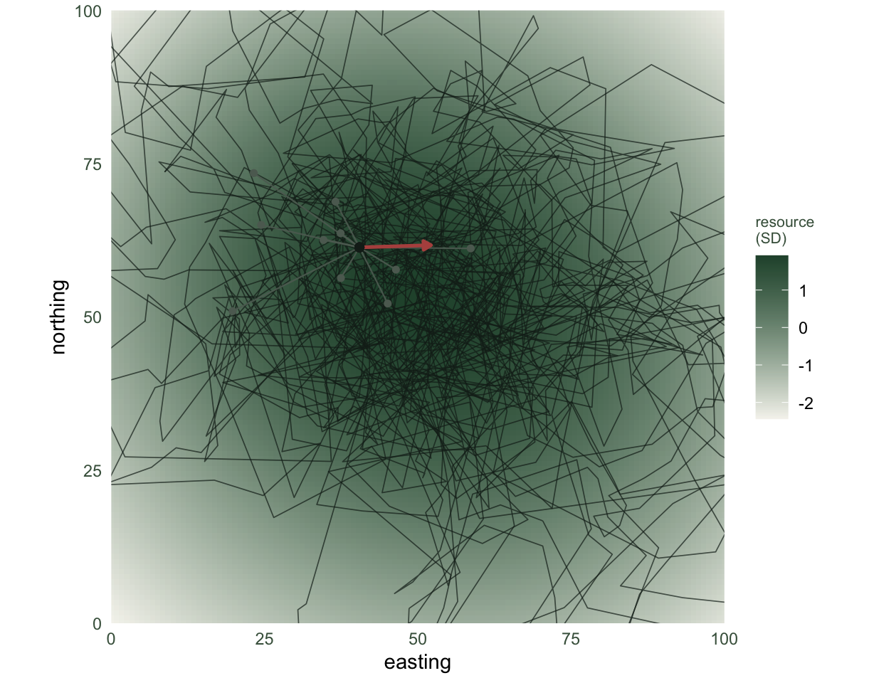
The conditional likelihood, by hand
Within a stratum the animal chose the used step out of the K + 1 on offer. If selection is proportional to exp(z * beta), the probability that this particular step was the one taken is a softmax over the stratum:
\[ \Pr(\text{used}_s) = \frac{\exp(z_{s,\text{used}}\,\beta)}{\sum_{j} \exp(z_{s,j}\,\beta)} . \]
The starting location enters the numerator and every term of the denominator identically, so it cancels. That is the whole point: the local abundance of the resource, which differs from stratum to stratum, drops out, and what remains is the selection for the resource over and above what was locally available. Summing the log of this over strata gives the conditional log-likelihood, which we hand to optim.
clogit_nll <- function(b) {
  eta <- Z * b
  -sum(eta[, 1] - log(rowSums(exp(eta))))
}
opt <- optim(0, clogit_nll, method = "BFGS", hessian = TRUE,
             control = list(reltol = 1e-10))
b_hat <- opt$par
se_hat <- sqrt(1 / opt$hessian[1, 1])
ci <- b_hat + c(-1, 1) * 1.96 * se_hat
rss <- exp(b_hat)
The estimate is 0.741 with a standard error of 0.059 and a 95% interval of [0.63, 0.86]. Exponentiating gives the relative selection strength: exp(beta) is 2.1, so a step ending in a cell one standard deviation richer in the resource is about 2.1 times as likely as an otherwise identical step ending in an average cell. This estimator is a conditional logistic regression; equivalently it is a Cox proportional hazards model stratified by step, which is how most software fits it.
Why the strata are not optional
It is tempting to throw the used and available steps into one ordinary logistic regression with a single intercept and forget the pairing. That intercept has to stand for the average availability across the whole track, but availability is not constant: as the animal moves through richer and poorer parts of the surface, the resource near its current position rises and falls. A single intercept cannot follow it, and the selection coefficient absorbs the damage.
long_z <- as.vector(t(Z))
long_y <- rep(c(1, rep(0, K)), n_str)
g_pool <- glm(long_y ~ long_z, family = binomial)
b_pool <- unname(coef(g_pool)[2]); se_pool <- summary(g_pool)$coefficients[2, 2]
Pooling collapses the coefficient to 0.142, far below the conditional estimate. The signal has not weakened; it has been averaged away by an intercept that could not track the moving baseline. Conditioning on the stratum is what protects it.
Checking against the truth, and where the bias comes from
Because this is a simulation we know the answer, so we can check the method directly. We draw the available steps from the movement kernel that actually generated the track, rather than from a kernel fitted to the observed steps.
set.seed(424242)
Zctrl_true <- matrix(NA_real_, n_str, K)
for (s in seq_along(use_idx)) {
  i <- use_idx[s]
  Ls <- rgamma(K, shape = sh_move, scale = sc_move)
  as <- rvm(K, 0, kap_move)
  ang <- heading[i] + as
  Zctrl_true[s, ] <- resource(pos[i, 1] + Ls * cos(ang), pos[i, 2] + Ls * sin(ang))
}
Zt <- cbind(Zcase, Zctrl_true)
clogit_nll_t <- function(b) { eta <- Zt * b; -sum(eta[, 1] - log(rowSums(exp(eta)))) }
opt_t <- optim(0, clogit_nll_t, method = "BFGS", hessian = TRUE, control = list(reltol = 1e-10))
b_hat_true <- opt_t$par; se_hat_true <- sqrt(1 / opt_t$hessian[1, 1])
With the true movement kernel supplying availability the estimate is 0.854, against a generative value of 0.85. The fitted-kernel estimate above is 0.74, and where the two differ the reason is instructive: the tentative gamma and von Mises were fitted to the observed steps, but the observed steps are already the product of selection, so the availability distribution they imply is slightly wrong. Estimating the movement kernel and the habitat selection together, rather than fixing one and inferring the other, removes this bias. That is integrated step selection analysis, and it is the next post.
dens_df <- rbind(data.frame(kind = "used steps", z = Zcase),
                 data.frame(kind = "available steps", z = as.vector(Zctrl)))
pa <- ggplot(dens_df, aes(z, fill = kind, colour = kind)) +
  geom_density(alpha = 0.45, linewidth = 0.5) +
  scale_fill_manual(values = c("used steps" = "#275139", "available steps" = "#93a87f")) +
  scale_colour_manual(values = c("used steps" = "#275139", "available steps" = "#93a87f")) +
  labs(x = "resource at step endpoint (SD)", y = "density", fill = NULL, colour = NULL) +
  theme_minimal(base_size = 11) + te_canvas +
  theme(panel.grid.minor = element_blank(), legend.position = "inside", legend.position.inside = c(0.72, 0.85),
        legend.background = element_rect(fill = "#ffffff", colour = NA))
coef_df <- data.frame(
  model = factor(c("conditional: movement kernel", "conditional: fitted kernel",
                   "pooled: strata ignored"),
                 levels = c("pooled: strata ignored", "conditional: fitted kernel",
                            "conditional: movement kernel")),
  est = c(b_hat_true, b_hat, b_pool), se = c(se_hat_true, se_hat, se_pool))
pb <- ggplot(coef_df, aes(est, model)) +
  geom_vline(xintercept = beta_true, linetype = "dashed", colour = "#b5534e") +
  geom_errorbar(aes(xmin = est - 1.96 * se, xmax = est + 1.96 * se),
                orientation = "y", width = 0.16, colour = "#275139", linewidth = 0.6) +
  geom_point(colour = "#275139", size = 2.6) +
  annotate("text", x = beta_true, y = 3.44, label = "true beta",
           colour = "#b5534e", size = 3, hjust = 1.1) +
  labs(x = "selection coefficient", y = NULL) +
  theme_minimal(base_size = 11) + te_canvas + theme(panel.grid.minor = element_blank(),
                                                     plot.margin = margin(5.5, 12, 5.5, 5.5))
grid.newpage()
pushViewport(viewport(layout = grid.layout(1, 2, widths = unit(c(1, 1), "null"))))
print(pa, vp = viewport(layout.pos.row = 1, layout.pos.col = 1))
print(pb, vp = viewport(layout.pos.row = 1, layout.pos.col = 2))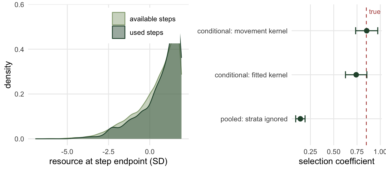
Selection at which scale
A step selection function and a resource selection function answer different questions, so their coefficients are not two estimates of one quantity. Here we fit a plain resource selection function on the same simulated data, with available points drawn from across the whole domain rather than from reachable steps.
set.seed(999)
used_pts <- trk[-1, ]
n_av <- nrow(used_pts) * K
av_pts <- data.frame(x = runif(n_av, 0, 100), y = runif(n_av, 0, 100))
rsf_y <- c(rep(1, nrow(used_pts)), rep(0, n_av))
rsf_z <- c(resource(used_pts$x, used_pts$y), resource(av_pts$x, av_pts$y))
g_rsf <- glm(rsf_y ~ rsf_z, family = binomial)
b_rsf <- unname(coef(g_rsf)[2])
The domain-wide resource selection function returns 0.65. It is not wrong, and it is not the same thing: it measures broad-scale use of the landscape, the tendency to end up in rich areas over the whole track, whereas the step selection coefficient measures the choice made at each move given where the animal already was. These are different orders of selection in the sense of Johnson (1980), and a study should be clear about which one it is asking for. The step scale is where movement and habitat interact, and it is where the next post puts them together.
Several animals: pooling individuals
Everything above is one animal. A study usually collars several, and the question it then asks is about the population: do these animals, on average, select for the resource? The conditional likelihood makes one answer easy, which is to stack every stratum of every animal into one fit and read off one coefficient and one standard error. That is a different pooling from the one earlier in this post: the strata are kept, and what is thrown away is the animal. If each animal has its own selection slope, drawn around a population mean with standard deviation sigma, the pooled fit treats a hundred steps of one animal as a hundred independent pieces of evidence about the mean, when they are a hundred pieces of evidence about that animal’s slope. The mechanism is the omitted random slope, which omitted random slopes and false positives measures for quadrats within grassland sites, and Muff, Signer and Fieberg (2020) compared random-slope step selection fits with fits that leave the slopes out and with a two-step approach; neither is repeated here. Two things matter more here than for quadrats in sites, because a collar delivers hundreds of steps per animal, and they are what this section measures on this post’s own strata: the damage grows with the number of steps per animal (that post held its quadrats at ten and showed that adding sites does not help), and the variance that sets it is the variance of the resource inside a stratum, not across the landscape, which is particular to the conditional likelihood.
Both follow from the score of the conditional likelihood at a slope of zero. For one step the score is the resource at the used step minus the mean over its stratum. If the animal’s own slope is beta_i, the expected score is close to beta_i * Vw, where Vw is the within-stratum variance of the resource, and its variance is Vw. Summed over the S steps of one animal, the score has variance S * Vw from the steps plus sigma^2 * S^2 * Vw^2 from the animal’s slope, and the pooled fit counts only the first. The ratio is the design effect of a cluster sample with the animal as the cluster, DE = 1 + sigma^2 * S * Vw, and a 5 per cent Wald test of a true mean slope of zero then rejects with probability 2 * pnorm(-1.96 / sqrt(DE)). The number of animals does not appear. With unequal step counts, S becomes sum(S_i^2) / sum(S_i), so one long track dominates.
To check this without leaving the post, each simulated animal reuses the strata of the track above. For every step one of the 1199 strata of Z is drawn at random, its 11 resource values become the candidates (the host’s used step counts as one more candidate), and the animal picks one with probability proportional to exp(beta_i * z). The slopes beta_i are normal with mean zero, so every rejection is a false positive. Each dataset gets four tests: the pooled fit with its usual standard error; the same fit with a sandwich standard error, clustered by animal and built from each animal’s summed score; a two-stage test, with one conditional fit per animal and a one-sample t test on the animal slopes with I - 1 degrees of freedom; and a precision-weighted two-stage z test, in which the animal slopes are weighted by the inverse of their variance plus a between-animal variance (the DerSimonian-Laird estimator). Every fit maximises this post’s conditional likelihood, by Newton steps rather than optim for speed; the mgcv chunk further down checks that the two agree. The design (5 and 20 animals, 25 to 400 steps, sigma 0.5 and 0, 1000 or 2000 datasets per cell) was fixed before anything was run.
# within-stratum variance of the resource on this track, and its total variance
vw_host <- mean(rowMeans((Z - rowMeans(Z))^2))
var_host <- var(as.vector(Z))
vw_iid <- K / (K + 1)            # K + 1 independent standard normal candidates
herd_de <- function(sig_b, steps, vw) 1 + sig_b^2 * steps * vw
herd_rej <- function(de) 2 * pnorm(-qnorm(0.975) / sqrt(de))

# n_anim animals with slopes N(mu_b, sig_b); each step reuses one stratum of Z
draw_herd <- function(n_anim, steps, mu_b, sig_b) {
  if (length(steps) == 1) steps <- rep(steps, n_anim)
  b_anim <- rnorm(n_anim, mu_b, sig_b)
  who <- rep(seq_len(n_anim), steps)
  zz <- Z[sample.int(nrow(Z), length(who), replace = TRUE), , drop = FALSE]
  gumbel <- -log(-log(matrix(runif(length(zz)), nrow(zz))))
  pick <- max.col(zz * b_anim[who] + gumbel, ties.method = "first")
  rc <- cbind(seq_len(nrow(zz)), pick)
  used <- zz[rc]; zz[rc] <- zz[, 1]; zz[, 1] <- used   # used step to column 1
  list(z = zz, who = who, steps = steps)
}

# the conditional likelihood of this post, maximised by Newton steps,
# one slope per group (a single group is the pooled fit)
clogit_newton <- function(zz, grp, n_grp) {
  bb <- numeric(n_grp)
  for (it in 1:40) {
    ee <- exp(zz * bb[grp]); pr <- ee / rowSums(ee)
    m1 <- rowSums(pr * zz); m2 <- rowSums(pr * zz^2)
    stp <- unname(rowsum(zz[, 1] - m1, grp)[, 1] / rowsum(m2 - m1^2, grp)[, 1])
    bb <- bb + stp
    if (max(abs(stp)) < 1e-10) break
  }
  ee <- exp(zz * bb[grp]); pr <- ee / rowSums(ee)
  m1 <- rowSums(pr * zz); m2 <- rowSums(pr * zz^2)
  list(b = bb, info = unname(rowsum(m2 - m1^2, grp)[, 1]), score = zz[, 1] - m1)
}

# inverse-variance weights plus a between-animal variance (DerSimonian-Laird)
dl_pool <- function(b_i, se_i) {
  w0 <- 1 / se_i^2; b_fix <- sum(w0 * b_i) / sum(w0)
  q_stat <- sum(w0 * (b_i - b_fix)^2)
  tau2 <- max(0, (q_stat - (length(b_i) - 1)) / (sum(w0) - sum(w0^2) / sum(w0)))
  w1 <- 1 / (se_i^2 + tau2)
  c(est = sum(w1 * b_i) / sum(w1), se = 1 / sqrt(sum(w1)), tau2 = tau2)
}

herd_rep <- function(n_anim, steps, sig_b) {
  hd <- draw_herd(n_anim, steps, 0, sig_b)
  pf <- clogit_newton(hd$z, rep(1L, nrow(hd$z)), 1)
  se_rob <- sqrt(sum(rowsum(pf$score, hd$who)^2)) / pf$info
  af <- clogit_newton(hd$z, hd$who, n_anim)
  dl <- dl_pool(af$b, 1 / sqrt(af$info))
  c(b = pf$b, z_pool = pf$b * sqrt(pf$info), z_rob = pf$b / se_rob,
    t_two = mean(af$b) / (sd(af$b) / sqrt(n_anim)), z_dl = dl[["est"]] / dl[["se"]],
    inv_info = 1 / pf$info, s_eff = sum(hd$steps^2) / sum(hd$steps))
}

herd_rates <- function(n_rep, n_anim, steps, sig_b) {
  rr <- t(replicate(n_rep, herd_rep(n_anim, if (is.function(steps)) steps() else steps, sig_b)))
  zc <- qnorm(0.975)
  data.frame(n_anim = n_anim, steps = mean(rr[, "s_eff"]), sig_b = sig_b, n_rep = n_rep,
             pool = mean(abs(rr[, "z_pool"]) > zc), rob = mean(abs(rr[, "z_rob"]) > zc),
             two = mean(abs(rr[, "t_two"]) > qt(0.975, n_anim - 1)),
             dl = mean(abs(rr[, "z_dl"]) > zc),
             de_var = var(rr[, "b"]) / mean(rr[, "inv_info"]),
             formula = mean(herd_rej(herd_de(sig_b, rr[, "s_eff"], vw_host))))
}

set.seed(26092601)
herd_plan <- data.frame(n_anim = c(5, 5, 20, 5, 5, 5, 5, 20),
                        steps  = c(100, 100, 100, 25, 50, 200, 400, 25),
                        sig_b  = c(0.5, 0, 0.5, 0.5, 0.5, 0.5, 0.5, 0.5),
                        n_rep  = c(2000, 2000, 1000, 1000, 1000, 1000, 1000, 1000))
herd_tab <- do.call(rbind, lapply(seq_len(nrow(herd_plan)), function(r)
  with(herd_plan[r, ], herd_rates(n_rep, n_anim, steps, sig_b))))
herd_uneq <- herd_rates(2000, 5, function() sample(20:200, 5, replace = TRUE), 0.5)
herd_tab$mc_se <- sqrt(herd_tab$pool * (1 - herd_tab$pool) / herd_tab$n_rep)

herd_cell <- function(a, s, g) herd_tab[herd_tab$n_anim == a & herd_tab$steps == s & herd_tab$sig_b == g, ]
h_main <- herd_cell(5, 100, 0.5); h_null <- herd_cell(5, 100, 0); h_20 <- herd_cell(20, 100, 0.5)
h_25a <- herd_cell(5, 25, 0.5); h_25b <- herd_cell(20, 25, 0.5); h_400 <- herd_cell(5, 400, 0.5)
h_sig <- herd_tab[herd_tab$sig_b == 0.5 & herd_tab$n_anim == 5, ]
rej_sand <- function(n_anim) 2 * pt(-qnorm(0.975) * sqrt((n_anim - 1) / n_anim), n_anim - 1)
rej_zt <- function(n_anim) 2 * pt(-qnorm(0.975), n_anim - 1)
# Monte Carlo standard error of the measured variance design effect (normal theory)
de_var_se <- h_main$de_var * sqrt(2 / (h_main$n_rep - 1))
de_gap <- abs(h_main$de_var - herd_de(0.5, 100, vw_host))
stopifnot(de_gap < de_var_se)
On this track Vw is 0.300, averaged over the strata, while the resource varies with variance 1.71 over all the step endpoints: the candidates in one stratum start from the same point and a step does not reach far on a smooth surface, so each stratum sees a narrow slice of the resource. For K + 1 independent standard normal candidates, the simplest construction, Vw would be K / (K + 1) = 0.909. At sigma 0.5 and 100 steps per animal the formula gives a design effect of 8.51 and a false positive rate of 0.502 on these strata, against 0.687 with independent candidates. That 0.687, about two false positives in three, belongs to that construction, not to step selection in general; how large Vw is depends on how far the available steps reach relative to the grain of the resource. Animals followed for as long as the track above (1199 steps) would push the formula to 0.837, whatever their number; that value was not simulated.
With five animals of 100 steps and sigma 0.5, the pooled fit rejects the true null in 0.505 of 2000 datasets (Monte Carlo standard error 0.011), where the formula gives 0.502: this reproduces the cluster design effect by simulation. With twenty animals of 100 steps the rate is 0.509, and at 25 steps it is 0.260 with five animals and 0.264 with twenty. Quadrupling the animals leaves the rate where it was; quadrupling the steps per animal raises it, to 0.723 at 400 steps. More data of the kind a collar produces makes the pooled test worse. The design effect on the variance of the pooled estimate is a different quantity from the rejection rate: measured as the variance of the estimates over the mean of their model-based variances it is 8.27 against the formula’s 8.51, a difference of 0.24 that is smaller than the Monte Carlo standard error of the measured ratio (about 0.26, from the sampling variance of a variance over 2000 datasets), and across the five step counts the formula predicts the rejection rate within 0.012. With unequal tracks (each animal’s step count drawn between 20 and 200) the pooled rate is 0.551, and the formula with sum(S_i^2) / sum(S_i) in place of S (on average 130) gives 0.546. Without any variation between animals (sigma 0) the pooled fit is honest, at 0.041 (Monte Carlo standard error 0.004).
curve_df <- data.frame(steps = exp(seq(log(20), log(450), length.out = 120)))
curve_df$this_track <- herd_rej(herd_de(0.5, curve_df$steps, vw_host))
curve_df$independent <- herd_rej(herd_de(0.5, curve_df$steps, vw_iid))
sig_tab <- herd_tab[herd_tab$sig_b == 0.5, ]
pts_df <- rbind(
  data.frame(steps = sig_tab$steps * ifelse(sig_tab$n_anim == 20, 1.06, 1),  # nudge right
             rate = sig_tab$pool, se = sig_tab$mc_se,
             test = ifelse(sig_tab$n_anim == 5, "pooled, 5 animals", "pooled, 20 animals")),
  data.frame(steps = h_sig$steps, rate = h_sig$rob, se = NA, test = "sandwich, 5 animals"),
  data.frame(steps = h_sig$steps, rate = h_sig$two, se = NA, test = "two-stage t, 5 animals"))
pts_df$test <- factor(pts_df$test, levels = c("pooled, 5 animals", "pooled, 20 animals",
                                              "sandwich, 5 animals", "two-stage t, 5 animals"))
ggplot() +
  geom_hline(yintercept = 0.05, colour = "#2c3a31", linetype = "dotted", linewidth = 0.5) +
  geom_line(data = curve_df, aes(steps, independent), colour = "#8a9a8f",
            linetype = "dashed", linewidth = 0.6) +
  geom_line(data = curve_df, aes(steps, this_track), colour = "#275139", linewidth = 0.8) +
  geom_errorbar(data = pts_df[!is.na(pts_df$se), ],
                aes(steps, ymin = rate - 2 * se, ymax = rate + 2 * se, colour = test),
                width = 0.04, linewidth = 0.5) +
  geom_point(data = pts_df, aes(steps, rate, colour = test, shape = test), size = 2.4) +
  annotate("text", x = 150, y = herd_rej(herd_de(0.5, 150, vw_iid)) + 0.06,
           label = "independent candidates", colour = "#5d6b61", size = 3, hjust = 1) +
  annotate("text", x = 140, y = herd_rej(herd_de(0.5, 140, vw_host)) - 0.07,
           label = "this track", colour = "#275139", size = 3, hjust = 0) +
  scale_x_log10(breaks = c(25, 50, 100, 200, 400)) +
  scale_colour_manual(values = c("#275139", "#b5534e", "#c9b458", "#16241d"), name = NULL) +
  scale_shape_manual(values = c(16, 17, 15, 18), name = NULL) +
  scale_y_continuous(limits = c(0, 0.9), breaks = seq(0, 0.9, 0.1)) +
  labs(x = "steps per animal (log scale)", y = "false positive rate") +
  theme_minimal(base_size = 11) + te_canvas +
  theme(panel.grid.minor = element_blank(), legend.position = "bottom",
        axis.text = element_text(colour = "#46604a")) +
  guides(colour = guide_legend(nrow = 2), shape = guide_legend(nrow = 2))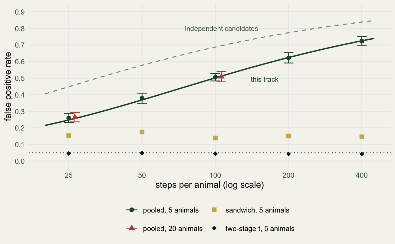
The two-stage t test holds its level at every step count, between 0.043 and 0.049 over all cells (and 0.038 with unequal tracks). It pays for this with I - 1 degrees of freedom, four with five animals, which is the honest amount of information about a population mean from five animals. The sandwich standard error is the usual first repair and it does not hold with five animals: 0.140 at sigma 0.5 and 0.144 with no variation between animals at all, 0.172 with unequal tracks. A sandwich variance is a variance estimated from five animal totals, divided by the number of animals rather than one fewer and read against a normal distribution, so with no heterogeneity it rejects with probability 2 * pt(-1.96 * sqrt(4/5), 4) = 0.154. Cluster bootstrap at six sites, and what beats it measures the same few-cluster failure for a site-level treatment. The precision-weighted two-stage z test sits between the two: 0.108 with five animals, more than twice the nominal level (a t statistic on four degrees of freedom read against a normal reference would reject in 0.122), and 0.069 with twenty (against 0.065).
That precision-weighted estimate matters because a random slope model returns something close to it; the one dataset below shows this, and it is not a result of the paper cited next. Klappstein et al. (2024) write step selection functions as penalised smooths in mgcv, where a random slope for each animal is the smooth s(x, id, bs = "re") and the conditional likelihood is the stratified Cox model mentioned after the hand-written likelihood above: family = cox.ph() with a two-column response of event time and stratum index, and the used indicator as the weight. That dataset has five animals with step counts from 30 to 250, a mean slope equal to this post’s beta_true and sigma 0.5.
library(mgcv)
set.seed(26092602)
demo_steps <- c(30, 60, 100, 160, 250)
demo <- draw_herd(5, demo_steps, beta_true, 0.5)
n_demo <- nrow(demo$z)
demo_long <- data.frame(stratum = rep(seq_len(n_demo), times = K + 1),
                        used = rep(c(1, rep(0, K)), each = n_demo),
                        x = as.vector(demo$z),
                        id = factor(rep(demo$who, times = K + 1)),
                        one = 1)

# pooled: this post's likelihood with optim, and the Newton version used above
clogit_nll_herd <- function(b, zz) { eta <- zz * b; -sum(eta[, 1] - log(rowSums(exp(eta)))) }
opt_demo <- optim(0, clogit_nll_herd, zz = demo$z, method = "BFGS", hessian = TRUE,
                  control = list(reltol = 1e-10))
nt_demo <- clogit_newton(demo$z, rep(1L, n_demo), 1)
stopifnot(abs(opt_demo$par - nt_demo$b) < 1e-5)

# mgcv: the second response column is read as the stratum index
gam_strat <- gam(cbind(one, stratum) ~ x, family = cox.ph(), weights = used, data = demo_long)
gam_flat <- gam(one ~ x, family = cox.ph(), weights = used, data = demo_long)
stopifnot(abs(coef(gam_strat)[["x"]] - nt_demo$b) < 1e-6,
          abs(sqrt(vcov(gam_strat)["x", "x"]) - 1 / sqrt(nt_demo$info)) < 1e-6)

# a random slope for each animal
gam_re <- gam(cbind(one, stratum) ~ x + s(x, id, bs = "re"), family = cox.ph(),
              weights = used, data = demo_long, method = "REML")
re_row <- summary(gam_re)$p.table["x", ]
invisible(capture.output(re_vc <- gam.vcomp(gam_re)))
# gam.vcomp() returns the standard deviations with intervals as a matrix (mgcv 1.9-1), as the
# vc element of a list (mgcv 1.9-4), or as a plain vector when it cannot form intervals
re_vm <- if (is.list(re_vc)) re_vc$vc else re_vc
re_sd <- as.numeric(if (is.matrix(re_vm)) re_vm[1, "std.dev"] else re_vm[1])
af_demo <- clogit_newton(demo$z, demo$who, 5)
dl_demo <- dl_pool(af_demo$b, 1 / sqrt(af_demo$info))
two_demo <- c(est = mean(af_demo$b), se = sd(af_demo$b) / sqrt(5))
demo_w <- 1 / (1 / af_demo$info + dl_demo[["tau2"]]); demo_w <- demo_w / sum(demo_w)
stopifnot(abs(re_row[["Pr(>|z|)"]] - 2 * pnorm(-abs(re_row[["z value"]]))) < 1e-10,
          which.min(af_demo$b) == 1)
# the weighted standard error with the REML between-animal variance plugged in
se_w_reml <- 1 / sqrt(sum(1 / (1 / af_demo$info + re_sd^2)))
stopifnot(abs(se_w_reml - re_row[["Std. Error"]]) < 5e-4)
p_t4 <- 2 * pt(-abs(re_row[["z value"]]), 4)
Without the random slope, the stratified mgcv fit reproduces this post’s conditional likelihood: 0.749867 against 0.749867 by hand, with the same standard error to six decimals (the chunk stops if not). Leave out the stratum column and the same call returns 0.140, the same collapse as in the section on why the strata are not optional. The pooled 0.750 has a standard error of 0.087. With the random slope the mean slope is 0.788 (standard error 0.174), the estimated standard deviation between animals 0.32 against a true 0.5, and the animal slopes themselves run from 0.10 to 1.35. The precision-weighted two-stage estimate is 0.783 (standard error 0.161) and the plain mean of the five slopes 0.775 (0.215): the random slope fit is 0.005 from the weighted estimate and 0.013 from the plain mean. Its standard error is 1.08 times the weighted one, because REML puts the between-animal standard deviation at 0.32 where DerSimonian-Laird puts it at 0.28; with the REML value in the weights, the weighted standard error is 0.174. The weights follow each animal’s precision, and the animal with 30 steps, which has the lowest slope, carries 0.13 of the weight and the one with 250 steps 0.27, against 0.20 each in the plain mean. The summary’s p value, 0.000006, reads the z value against a normal distribution; against a t distribution on four degrees of freedom the same z gives 0.011. The normal reference is what over-rejects with five animals in the simulation above (the weighted two-stage z test there), so the t reference on the number of animals minus one is the safer reading, as a heuristic rather than an exact small-sample correction.
The limits of this section are those of its construction. The simulated animals reuse strata of one track, so their steps are independent draws from this post’s availability, with no serial dependence between steps and no difference in home range or availability between animals, which real collars have. The animal slopes are normal and unrelated to anything the animal does, and the random slope mgcv fit was run once here, not replicated, so its error rate is read from the weighted two-stage test it approximates, not measured directly. What to report follows from the formula: the number of animals, the steps per animal, and a test whose degrees of freedom come from the animals rather than the steps.
References
Fortin D, Beyer HL, Boyce MS, Smith DW, Duchesne T, Mao JS 2005. Ecology 86(5):1320-1330 (10.1890/04-0953).
Thurfjell H, Ciuti S, Boyce MS 2014. Movement Ecology 2:4 (10.1186/2051-3933-2-4).
Forester JD, Im HK, Rathouz PJ 2009. Ecology 90(12):3554-3565 (10.1890/08-0874.1).
Johnson DH 1980. Ecology 61(1):65-71 (10.2307/1937156).
Manly BFJ, McDonald LL, Thomas DL, McDonald TL, Erickson WP 2002. Resource Selection by Animals, 2nd edn. Kluwer (ISBN 978-1-4020-0677-7).
Best DJ, Fisher NI 1979. Journal of the Royal Statistical Society Series C 28(2):152-157 (10.2307/2346732).
Muff S, Signer J, Fieberg J 2020. Journal of Animal Ecology 89(1):80-92 (10.1111/1365-2656.13087).
Klappstein NJ, Michelot T, Fieberg J, Pedersen EJ, Mills Flemming J 2024. Methods in Ecology and Evolution 15(8):1332-1346 (10.1111/2041-210x.14367).