library(ggplot2)
library(patchwork)

te_paper  <- "#f5f4ee"
te_ink    <- "#16241d"
te_body   <- "#2c3a31"
te_forest <- "#275139"
te_rust   <- "#b5534e"
te_gold   <- "#c9b458"
te_line   <- "#dad9ca"

theme_datasheet <- function() {
  theme_minimal(base_size = 12) +
    theme(plot.background  = element_rect(fill = te_paper, colour = NA),
          panel.background = element_rect(fill = te_paper, colour = NA),
          panel.grid.major = element_line(colour = te_line, linewidth = 0.3),
          panel.grid.minor = element_blank(),
          text             = element_text(colour = te_body),
          plot.title       = element_text(colour = te_ink, face = "bold"),
          plot.subtitle    = element_text(colour = te_body),
          axis.text        = element_text(colour = te_body))
}Cluster bootstrap at six sites, and what beats it
R
bootstrap
resampling
experimental design
pseudoreplication
simulation
ecology tutorial
At six catchments the cluster bootstrap and sandwich errors over-reject a site-level treatment. Measuring in R why the six site means are the analysis.
Six headwater catchments, three of them fenced against deer and three left open, twelve vegetation subplots in each. The response is sapling height growth, the subplots number seventy-two, and the treatment is a property of the catchment: every subplot inside a fenced catchment is fenced. Paired-catchment and whole-catchment manipulations look like this almost by necessity, because a fence, a liming run or a felling coupe is laid on a catchment, not on a quadrat, and catchments are expensive. Hurlbert’s 1984 paper on pseudoreplication is about exactly this design, and the unit that counts is the catchment.
Most analysts now know not to run an ordinary regression on the seventy-two subplots. The question is what to reach for instead, and two posts on this site give answers that are right where they were measured. Bootstrapping dependent data showed that resampling whole sites instead of rows repairs a clustered standard error, with twenty sites; its own sentence is that “the cluster bootstrap does especially well because twenty sites give plenty of units to resample”. Dependent effect sizes in meta-analysis showed that a clustered sandwich interval, with its k/(k-1) correction read against a t distribution on k-1 degrees of freedom, already holds at eight studies, for an intercept. Ecology’s paired-catchment designs have six sites and a treatment that does not vary inside one, and in that corner both results stop being true.
Neither post is wrong, and this one does not contradict them. The meta-analysis post names its own limit in so many words: “That agreement at eight studies is a property of the easiest possible case and should not be generalised. There is one covariate here, an intercept”, and it goes on to say that a moderator unbalanced across studies drags the effective degrees of freedom below k-1. A treatment that is constant inside a cluster is a moderator of that kind, and even perfectly balanced, as here, it has a cost that gets a closed form below. The bootstrap post measured at twenty sites; the first section here runs its own procedure at ten, six and four.
The result itself is not new. Cameron, Gelbach and Miller 2008 showed with simulations of this kind that clustered sandwich tests over-reject with five to thirty clusters, and that bootstrap-t procedures, the wild cluster bootstrap with the null imposed among them, bring the rate back towards nominal; MacKinnon and Webb 2017 showed where that wild bootstrap in turn fails, when only a few clusters are treated; Donald and Lang 2007 showed that when the regressor of interest is constant within groups, a regression on the group means with its own small degrees of freedom is the correct test under normal group errors. This post is a demonstration of that literature in an ecological design, with one row the ecological posts have not priced: Random effects with too few levels already recommends “reporting the regression on the group means as the primary analysis” for a covariate constant within groups, and the site-means row below measures that advice against every resampling scheme on the same data sets.
The same bootstrap, walked down from twenty sites
The bootstrap post’s clustered example has twenty sites, eight plots per site, a site standard deviation of one, a residual standard deviation of one and a true grand mean of five. It resamples rows or whole sites four hundred times and takes the percentile interval. The chunk below is that procedure, vectorised, with the number of sites as an argument. Each cell is five seed blocks of four hundred data sets, where that post ran seven hundred once, and the design constants were fixed before any cell was run.
cover_mean <- function(G, n_plot = 8, tau = 1, sigma = 1, mu = 5,
                       n_sets = 400, n_boot = 400) {
  hit_row <- 0; hit_site <- 0; N <- G * n_plot
  site <- rep(seq_len(G), each = n_plot)
  for (r in seq_len(n_sets)) {
    y <- mu + rnorm(G, 0, tau)[site] + rnorm(N, 0, sigma)
    site_mean <- as.vector(rowsum(y, site)) / n_plot
    pick <- matrix(sample.int(G, G * n_boot, TRUE), G, n_boot)
    boot_site <- colMeans(matrix(site_mean[pick], G, n_boot))  # whole sites
    boot_row  <- colMeans(matrix(sample(y, N * n_boot, TRUE), N, n_boot))
    ci_site <- quantile(boot_site, c(0.025, 0.975), names = FALSE)
    ci_row  <- quantile(boot_row,  c(0.025, 0.975), names = FALSE)
    hit_site <- hit_site + (mu >= ci_site[1] & mu <= ci_site[2])
    hit_row  <- hit_row  + (mu >= ci_row[1]  & mu <= ci_row[2])
  }
  c(row = hit_row / n_sets, site = hit_site / n_sets)
}
g_walk <- c(20, 10, 6, 4); n_block <- 5
walk <- do.call(rbind, lapply(g_walk, function(G) {
  out <- t(vapply(seq_len(n_block), function(k) {
    set.seed(77000 + 100 * G + k); cover_mean(G)
  }, numeric(2)))
  data.frame(G = G, block = seq_len(n_block), row = out[, "row"], site = out[, "site"])
}))
walk_sum <- function(G, col) {
  v <- walk[walk$G == G, col]; c(med = median(v), lo = min(v), hi = max(v))
}
w20 <- walk_sum(20, "site"); w10 <- walk_sum(10, "site")
w6 <- walk_sum(6, "site"); w4 <- walk_sum(4, "site")
r20 <- walk_sum(20, "row"); r4 <- walk_sum(4, "row")
At twenty sites the cluster interval covers the true mean in a median 0.927 of data sets across the five blocks (range 0.912 to 0.938), against 0.650 for the row bootstrap. That is the bootstrap post’s result reproduced: the row bootstrap resamples the wrong unit, and the site bootstrap repairs most of the shortfall. Walked down, the site interval covers 0.895 at ten sites, 0.860 at six and 0.800 at four, with block ranges of 0.825 to 0.887 at six sites. The row bootstrap sits at 0.598 at four sites. The site bootstrap is still far better than the row bootstrap at every size, and at six sites it is still a nominal ninety-five per cent interval that misses more than twice as often as it says.
walk_long <- rbind(data.frame(G = walk$G, cover = walk$row, unit = "resample rows"),
                   data.frame(G = walk$G, cover = walk$site, unit = "resample whole sites"))
walk_med <- aggregate(cover ~ G + unit, data = walk_long, FUN = median)
ggplot(walk_long, aes(G, cover, colour = unit)) +
  geom_hline(yintercept = 0.95, linetype = "dashed", colour = te_body, linewidth = 0.5) +
  geom_point(size = 1.4, alpha = 0.6) +
  geom_line(data = walk_med, linewidth = 0.9) +
  geom_point(data = walk_med, size = 2.6) +
  scale_x_continuous(breaks = g_walk) +
  scale_y_continuous(limits = c(0.5, 1)) +
  scale_colour_manual(values = c(te_rust, te_forest), name = NULL) +
  labs(x = "sites", y = "coverage of the 95 per cent interval",
       title = "Twenty sites is where the site bootstrap works",
       subtitle = "small points: five seed blocks of 400 data sets; large points: block medians") +
  theme_datasheet() + theme(legend.position = "bottom")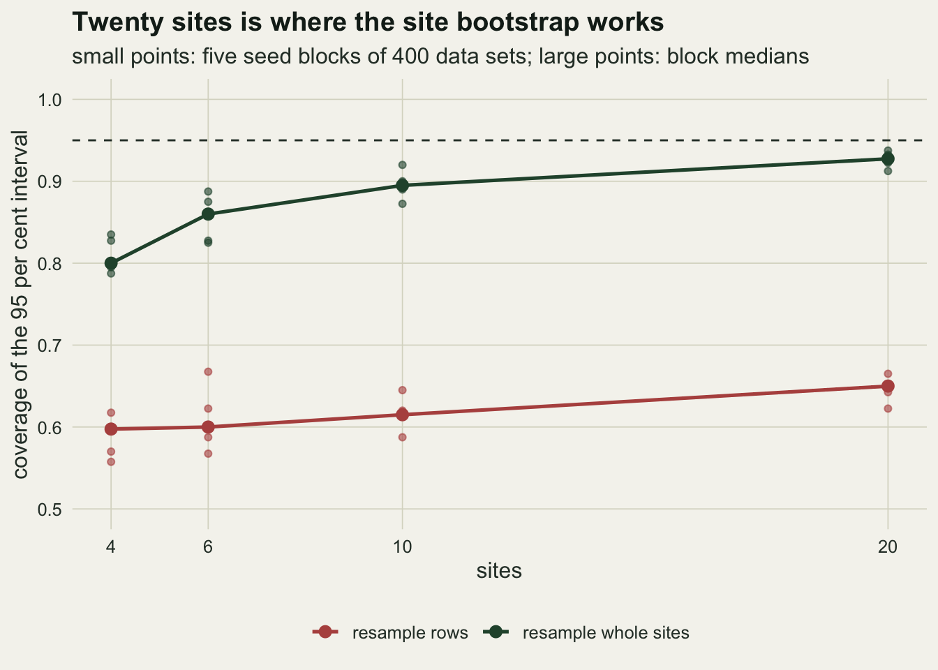
The quantity here is a grand mean, and the design has no treatment. The catchment study asks about a difference between fenced and open catchments, which is where the choice of reference distribution starts to matter more than the choice of resampling unit.
Six catchments, one slope, seven reference distributions
The design for the rest of the post: G catchments, half fenced, twelve subplots each, a catchment effect with standard deviation 0.6, a residual standard deviation of one, and no treatment effect at all. The estimate is the ordinary least squares slope on the fence indicator, which in a balanced design is the difference between the mean of the fenced catchment means and the mean of the open ones. Everything below is a different way of deciding whether that one number is far from zero.
Because the fence is constant inside a catchment and every catchment has twelve subplots, every statistic used here depends on the data only through the catchment means and, for the naive test, the within-catchment sum of squares. The functions work on the catchment means directly. That is a claim, so the first chunk checks it against the textbook matrix sandwich on the full subplot data.
n_plot <- 12; tau_site <- 0.6; sigma_plot <- 1; alpha_lev <- 0.05

gen_catch <- function(G, beta = 0) {
  fenced <- rep(c(0, 1), each = G / 2)
  site <- rep(seq_len(G), each = n_plot)
  y <- beta * fenced[site] + rnorm(G, 0, tau_site)[site] + rnorm(G * n_plot, 0, sigma_plot)
  site_mean <- as.vector(rowsum(y, site)) / n_plot
  list(y = y, site = site, fenced = fenced, site_mean = site_mean,
       ss_within = sum((y - site_mean[site])^2), G = G, N = G * n_plot)
}

# slope and CR1 sandwich variance from catchment means, one column per data version
cr1_cols <- function(mm, aa, G, N) {
  n1 <- colSums(aa); n0 <- G - n1
  m1 <- colSums(mm * aa) / n1; m0 <- colSums(mm * (1 - aa)) / n0
  dev <- mm - (aa * rep(m1, each = G) + (1 - aa) * rep(m0, each = G))
  v0 <- colSums(dev^2 * aa) / n1^2 + colSums(dev^2 * (1 - aa)) / n0^2
  list(b = m1 - m0, v = G / (G - 1) * (N - 1) / (N - 2) * v0)
}

set.seed(5106)
ex <- gen_catch(6)
xmat <- cbind(1, ex$fenced[ex$site])
xtx_inv <- solve(crossprod(xmat))
b_full <- xtx_inv %*% crossprod(xmat, ex$y)
score <- rowsum(as.vector(ex$y - xmat %*% b_full) * xmat, ex$site)
v_full <- 6 / 5 * (ex$N - 1) / (ex$N - 2) * (xtx_inv %*% crossprod(score) %*% xtx_inv)
ex_fit <- cr1_cols(matrix(ex$site_mean), matrix(ex$fenced), 6, ex$N)
sandwich_gap <- max(abs(c(b_full[2] - ex_fit$b, v_full[2, 2] - ex_fit$v)))
ex_t_cr <- ex_fit$b / sqrt(ex_fit$v)
On one simulated six-catchment data set the slope is -0.1292 and the two routes to the CR1 sandwich agree to within floating-point rounding. CR1 is the cluster sandwich with the usual small-sample factor, G/(G-1) times (N-1)/(N-2), the version most software prints by default.
The seven reference distributions, all applied to the same slope:
- The naive t test from the regression on all subplots, on N-2 degrees of freedom.
- The CR1 sandwich t statistic against a standard normal.
- The same statistic against t on G-1 degrees of freedom, which is the meta-analysis post’s recipe.
- The pairs cluster bootstrap: resample whole catchments with replacement 499 times, refit the slope, reject when the 95 per cent percentile interval excludes zero. A resample that draws only fenced or only open catchments has no slope; it is counted and left out of the interval.
- The studentised version of the same bootstrap, which refits the CR1 statistic in every resample and compares the observed statistic with the 95th percentile of the absolute resampled ones.
- The wild cluster bootstrap with the null imposed: fit the model without the fence, multiply each catchment’s residuals by a random sign, rebuild the response, refit the CR1 statistic. At G of ten or fewer every one of the 2^G sign patterns is used, so there is no bootstrap noise; above ten, 999 random patterns.
- The site-means t test: a two-sample t test with pooled variance on the G catchment means, on G-2 degrees of freedom.
sign_patterns <- function(G, n_rand = 999L) {
  if (G <= 10) t(as.matrix(expand.grid(rep(list(c(-1, 1)), G))))
  else matrix(sample(c(-1, 1), G * n_rand, TRUE), G, n_rand)
}
sp_fixed <- list("6" = sign_patterns(6), "10" = sign_patterns(10))

wild_t <- function(site_mean, fenced, G, N, spat) {
  grand <- mean(site_mean)                       # the fit with the null imposed
  mw <- grand + (site_mean - grand) * spat
  fw <- cr1_cols(mw, matrix(fenced, G, ncol(spat)), G, N)
  fw$b / sqrt(fw$v)
}

run_set <- function(G, beta = 0, n_boot = 499L) {
  d <- gen_catch(G, beta); N <- d$N; mbar <- d$site_mean; arm <- d$fenced
  fit <- cr1_cols(matrix(mbar), matrix(arm), G, N)
  b_hat <- fit$b; t_cr <- b_hat / sqrt(fit$v)
  arm_mean <- ifelse(arm == 1, mean(mbar[arm == 1]), mean(mbar[arm == 0]))
  ss_between <- sum((mbar - arm_mean)^2)
  se_ols <- sqrt((d$ss_within + n_plot * ss_between) / (N - 2) * 4 / N)
  se_means <- sqrt(ss_between / (G - 2) * 4 / G)
  # pairs cluster bootstrap, plain and studentised
  pick <- matrix(sample.int(G, G * n_boot, TRUE), G, n_boot)
  mb <- matrix(mbar[pick], G, n_boot); ab <- matrix(arm[pick], G, n_boot)
  n_f <- colSums(ab); usable <- n_f > 0 & n_f < G
  fb <- cr1_cols(mb[, usable, drop = FALSE], ab[, usable, drop = FALSE], G, N)
  ci <- quantile(fb$b, c(0.025, 0.975), names = FALSE)
  t_star <- abs(fb$b - b_hat) / sqrt(fb$v); t_star[fb$v <= 0] <- Inf
  crit_stud <- quantile(t_star, 0.95, names = FALSE)
  zero_var <- fb$v < 1e-12                      # both arms copies of one catchment
  crit_drop <- quantile(t_star[!zero_var], 0.95, names = FALSE)
  # wild cluster bootstrap, null imposed
  spat <- if (G <= 10) sp_fixed[[as.character(G)]] else sign_patterns(G)
  t_wild <- abs(wild_t(mbar, arm, G, N, spat))
  p_wild <- if (G <= 10) mean(t_wild >= abs(t_cr) * (1 - 1e-9)) else
    (1 + sum(t_wild >= abs(t_cr))) / (ncol(spat) + 1)
  c(naive  = abs(b_hat / se_ols) > qt(0.975, N - 2),
    cr1_z  = abs(t_cr) > qnorm(0.975),
    cr1_t  = abs(t_cr) > qt(0.975, G - 1),
    pairs  = ci[1] > 0 | ci[2] < 0,
    pairs_t = abs(t_cr) > crit_stud,
    pairs_t_drop = abs(t_cr) > crit_drop,
    wild   = p_wild <= alpha_lev,
    means  = abs(b_hat / se_means) > qt(0.975, G - 2),
    degen  = mean(!usable), p_wild = p_wild,
    sd_ratio = sd(fb$b) / se_means,
    hw_ratio = (ci[2] - ci[1]) / 2 / (qt(0.975, G - 2) * se_means),
    crit_stud = crit_stud, zero_share = mean(zero_var))
}
meth_key <- c("naive", "cr1_z", "cr1_t", "pairs", "pairs_t", "wild", "means")
meth_lab <- c("naive t, all subplots", "CR1 against normal", "CR1 against t(G-1)",
              "pairs cluster bootstrap", "studentised pairs bootstrap",
              "wild cluster bootstrap", "site-means t test")

set.seed(5106)
ex_one <- run_set(6)
ex_means <- t.test(ex$site_mean[ex$fenced == 1], ex$site_mean[ex$fenced == 0], var.equal = TRUE)
n_reject_ex <- sum(ex_one[meth_key])
The set.seed before run_set(6) reproduces the data set checked above, so the seven decisions are about that slope. On it, none of the seven procedures reject the null of no fence effect at five per cent. The site-means t test, which t.test confirms gives a p value of 0.811, does not reject either, and the wild bootstrap p value is 0.7500. One data set says nothing about error rates, so the next step is thousands of them.
Counting false alarms across the number of sites
Four catchment counts, six, ten, twenty and forty; at each, five seed blocks of four hundred null data sets. Block medians and ranges are reported so that the block-to-block noise stays visible.
g_grid <- c(6, 10, 20, 40); n_sets <- 400
sim_rows <- list(); keep_p6 <- NULL
for (G in g_grid) {
  for (k in seq_len(n_block)) {
    set.seed(1000 * G + k)
    out <- vapply(seq_len(n_sets), function(i) run_set(G), numeric(14))
    sim_rows[[length(sim_rows) + 1]] <- data.frame(G = G, block = k, t(rowMeans(out)))
    if (G == 6) keep_p6 <- rbind(keep_p6, t(out[c("p_wild", "sd_ratio", "hw_ratio", "crit_stud"), ]))
  }
}
sim_tab <- do.call(rbind, sim_rows)
rate_at <- function(G, key, f = median) f(sim_tab[sim_tab$G == G, key])
rng_txt <- function(G, key) sprintf("%.3f [%.3f, %.3f]", rate_at(G, key), rate_at(G, key, min),
                                    rate_at(G, key, max))
mcse_block <- sqrt(alpha_lev * (1 - alpha_lev) / n_sets)
mcse_pool  <- sqrt(alpha_lev * (1 - alpha_lev) / (n_block * n_sets))
gap_min6 <- rate_at(6, "pairs", min) - rate_at(6, "wild", max)
ratio6 <- rate_at(6, "pairs") / rate_at(6, "wild")
The Monte Carlo standard error of a rejection rate of five per cent is 0.0109 within a block and 0.0049 pooled over the 2000 data sets at one catchment count.
At six catchments, as median [lowest block, highest block]: the naive subplot regression rejects a true null at 0.340 [0.318, 0.365]. The CR1 sandwich read against a normal rejects at 0.150 [0.130, 0.163], and the same statistic read against t on five degrees of freedom at 0.083 [0.065, 0.085]. The pairs cluster bootstrap rejects at 0.170 [0.150, 0.200] and its studentised version at 0.007 [0.003, 0.007]. The wild cluster bootstrap rejects at 0.050 [0.037, 0.058], and the site-means t test at 0.050 [0.037, 0.055]. Those two hold the level equally well; what separates them comes later, in the floor section.
The pairs bootstrap and the wild bootstrap do not overlap in any block: the lowest pairs block is 0.092 above the highest wild block, and the median ratio is 3.4. The procedure the bootstrap post recommends, applied to the design the catchment study has, rejects a true null 3.4 times as often as the wild bootstrap does and more than three times the nominal rate.
At ten catchments the medians are 0.090 for CR1 against the normal, 0.052 against t, 0.095 for the pairs bootstrap, 0.048 for the wild bootstrap and 0.043 for the site means. At forty they are 0.065, 0.060, 0.070, 0.058 and 0.058. The naive subplot test never improves: across every block at every catchment count its rate stays between 0.297 and 0.370, because adding catchments does nothing about a test that counts subplots as replicates.
k_factor <- function(G, N = G * n_plot) sqrt((G - 1) * (N - 2) / ((G - 2) * (N - 1)))
cf_rate <- function(G, crit) 2 * pt(-crit / k_factor(G), G - 2)
cf_tab <- data.frame(G = rep(g_grid, 2),
                     key = rep(c("cr1_z", "cr1_t"), each = length(g_grid)),
                     rate = c(cf_rate(g_grid, qnorm(0.975)), cf_rate(g_grid, qt(0.975, g_grid - 1))))
cf_z6 <- cf_rate(6, qnorm(0.975)); cf_t6 <- cf_rate(6, qt(0.975, 5))
cf_dev <- vapply(seq_len(nrow(cf_tab)), function(i)
  mean(sim_tab[sim_tab$G == cf_tab$G[i], cf_tab$key[i]]) - cf_tab$rate[i], 0)
cf_gap <- max(abs(cf_dev))
cf_z <- max(abs(cf_dev) / sqrt(cf_tab$rate * (1 - cf_tab$rate) / (n_block * n_sets)))
ex_t_means <- unname(ex_means$statistic)
t_ratio_ex <- ex_t_cr / ex_t_means
The two sandwich rows have a closed form in this design, which is the bridge to the meta-analysis post. With a balanced two-arm treatment constant inside catchments, the CR1 variance is the pooled site-means variance multiplied by (G-2)/(G-1) and by (N-1)/(N-2), so the CR1 t statistic is the site-means t statistic times a fixed factor, 1.1101 at six catchments (on the example data set the ratio of the two statistics is 1.1101). The site-means statistic has an exact t distribution on G-2 degrees of freedom, so the rejection rate of each sandwich test is one call to pt: 0.152 against the normal and 0.082 against t(5) at six catchments. Across all eight sandwich cells the simulation and the closed form differ by at most 0.011, which in every cell is within 1.93 Monte Carlo standard errors of the closed-form rate.
For an intercept alone the same algebra gives a factor of exactly one: the CR1 statistic read against t(G-1) is then the one-sample t test on the site means. The meta-analysis post’s weighted mean is close to that equal-weight case, which is why its clustered interval came out close to target at eight studies. The treatment costs one degree of freedom that the t(G-1) reference does not charge, and it shrinks the sandwich by (G-2)/(G-1). At forty catchments neither matters; at six, the pair of them turns a five per cent test into one that rejects 8.2 per cent of the time.
long_rows <- lapply(seq_along(meth_key), function(j)
  data.frame(G = sim_tab$G, method = meth_lab[j], rate = sim_tab[[meth_key[j]]]))
long_tab <- do.call(rbind, long_rows)
sum_tab <- do.call(rbind, lapply(split(long_tab, list(long_tab$G, long_tab$method)), function(s)
  data.frame(G = s$G[1], method = s$method[1], med = median(s$rate),
             lo = min(s$rate), hi = max(s$rate))))
sum_tab$method <- factor(sum_tab$method, levels = meth_lab)
cf_plot <- data.frame(G = cf_tab$G, rate = cf_tab$rate,
                      method = factor(ifelse(cf_tab$key == "cr1_z", meth_lab[2], meth_lab[3]),
                                      levels = meth_lab))
meth_col <- c(te_body, te_gold, "#8a7a2e", te_rust, "#8fa898", te_forest, te_ink)
names(meth_col) <- meth_lab
shown <- sum_tab[sum_tab$method != meth_lab[1], ]
ggplot(shown, aes(G, med, colour = method)) +
  geom_hline(yintercept = alpha_lev, linetype = "dashed", colour = te_body, linewidth = 0.5) +
  geom_line(data = cf_plot, aes(G, rate), linewidth = 0.5, alpha = 0.7) +
  geom_errorbar(aes(ymin = lo, ymax = hi), width = 0, linewidth = 0.5,
                position = position_dodge(width = 2.4)) +
  geom_point(size = 2.3, position = position_dodge(width = 2.4)) +
  scale_x_continuous(breaks = g_grid) +
  scale_colour_manual(values = meth_col, name = NULL) +
  guides(colour = guide_legend(ncol = 2)) +
  labs(x = "catchments (half fenced, twelve subplots each)", y = "rejection rate under the null",
       title = "Few catchments, and the choice of reference is the result",
       subtitle = paste0("naive subplot test omitted: every block above ",
                         sprintf("%.2f", floor(100 * min(sim_tab$naive)) / 100))) +
  theme_datasheet() + theme(legend.position = "bottom")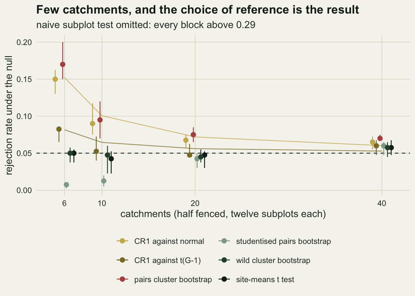
Why the pairs bootstrap runs hot, and its studentised version runs cold
The pairs bootstrap has no closed form, but its interval can be taken apart. For each null data set at six catchments, compare the spread of the resampled slopes with the site-means standard error, and compare the half-width of the percentile interval with the half-width of the site-means t interval.
sd6 <- median(keep_p6[, "sd_ratio"]); hw6 <- median(keep_p6[, "hw_ratio"])
crit_t4 <- qt(0.975, 4); eff_mult <- hw6 * crit_t4 / sd6
crit_stud6 <- median(keep_p6[, "crit_stud"])
inv_k6 <- 1 / k_factor(6); mult_ratio <- eff_mult / crit_t4
n_multisets <- choose(2 * 6 - 1, 6)
set.seed(4242)
arm6 <- rep(c(0, 1), each = 3)
pick6 <- matrix(sample.int(6, 6 * 1e5, TRUE), 6)
one_site_arm <- apply(pick6, 2, function(ix) {
  f <- ix[arm6[ix] == 1]; o <- ix[arm6[ix] == 0]
  ok <- length(f) > 0 && length(o) > 0
  c(any = ok && (length(unique(f)) == 1 || length(unique(o)) == 1),
    both = ok && length(unique(f)) == 1 && length(unique(o)) == 1)
})
share_one_site <- mean(one_site_arm["any", ])
share_both_site <- mean(one_site_arm["both", ])
zero_share6 <- rate_at(6, "zero_share", mean)
# the same property counted over the distinct resamples instead of the draws
ms6 <- unique(t(apply(as.matrix(expand.grid(rep(list(1:6), 6))), 1, sort)))
share_one_ms <- mean(apply(ms6, 1, function(ix) {
  f <- ix[arm6[ix] == 1]; o <- ix[arm6[ix] == 0]
  length(f) > 0 && length(o) > 0 && (length(unique(f)) == 1 || length(unique(o)) == 1)
}))
# bootstrap SD / site-means SE if the bootstrap were run to infinity:
# sqrt(E[1/n1*] * (G-2)/2), n1* = fenced draws given a usable resample
boot_sd_ideal <- function(G) {
  k <- seq_len(G - 1); w <- dbinom(k, G, 0.5)
  sqrt(sum(w / k) / sum(w) * (G - 2) / 2)
}
Across the two thousand data sets at six catchments the bootstrap standard deviation of the slope has a median of 0.900 times the site-means standard error. The sandwich’s shrinkage factor from the previous section is 0.901, so at six catchments the pairs bootstrap lands almost exactly on the CR1 standard error. That is a coincidence of this catchment count, not a shared mechanism: the bootstrap’s variance charges no degrees of freedom at all, and the random number of fenced catchments in each resample inflates it back up. Run to infinity, the bootstrap ratio would be 0.900 at six catchments against the sandwich’s 0.901, but 0.958 against 0.947 at ten. The percentile interval then spends that spread as if the reference were close to normal: its half-width is 0.607 times the site-means t half-width, which corresponds to a multiplier of about 1.87 bootstrap standard deviations, where the exact test uses 2.776 site-means standard errors, a ratio of 0.675. So the answer to whether the failure is the variance or the resampling is both, and the larger share is the reference: the percentile interval has no way to know that six catchments leave four degrees of freedom.
Studentising the bootstrap is the textbook fix for that, and at six catchments it overshoots. A resample whose fenced arm is made of copies of a single catchment has a within-arm spread of zero, so its CR1 variance is small and its t statistic large, and 0.420 of all resamples at six catchments have at least one arm like that (from 100000 resampled index sets). The median 95th percentile of the resampled absolute t statistics is 7.89, against a t(4) critical value of 2.776, and the test rejects at 0.007 [0.003, 0.007]. It holds its level by being far too cautious, and the power section below shows the price. That is the finite resample space showing through: six catchments drawn with replacement can form only 462 distinct resamples (462 counted directly), and 0.617 of them have a single-catchment arm. Such a resample repeats catchments, so it is drawn less often than one made of distinct catchments, which is why the share of draws, 0.420, is the lower of the two.
The wild bootstrap has a floor, and it is 1/32
The wild cluster bootstrap holds its level at six catchments, but it cannot say much. With six catchments and signs that are either plus or minus there are 2^6 = 64 sign patterns, and with the null imposed every one of them is a possible rebuilt data set. The pattern of all plus signs rebuilds the observed data exactly, so the observed statistic is always among the 64. The pattern of all minus signs rebuilds the data mirrored about the grand mean: the same statistic with its sign flipped.
pat6 <- sp_fixed[["6"]]
t64 <- wild_t(ex$site_mean, ex$fenced, 6, ex$N, pat6)
mirror_gap <- max(abs(abs(t64) - abs(wild_t(ex$site_mean, ex$fenced, 6, ex$N, -pat6))))
n_distinct <- length(unique(round(abs(t64), 8)))
p_floor6 <- 2 / 2^6; p_floor10 <- 2 / 2^10
p_tab <- as.data.frame(table(p = round(keep_p6[, "p_wild"] * 64)))
p_tab$p <- as.integer(as.character(p_tab$p)) / 64
p_tab$share <- p_tab$Freq / nrow(keep_p6)
share_floor <- mean(abs(keep_p6[, "p_wild"] - p_floor6) < 1e-9)
degen_cf6 <- 2 * 0.5^6; degen_cf10 <- 2 * 0.5^10
degen_sim6 <- mean(sim_tab$degen[sim_tab$G == 6])
n_odd <- sum(round(keep_p6[, "p_wild"] * 64) %% 2 == 1)
perm_n <- choose(6, 3); perm_floor <- 2 / perm_n
Every pattern and its mirror image give the same absolute statistic (on the example data set each of the 64 patterns matches its mirror to within floating-point rounding), so the 64 patterns carry 32 distinct absolute values. The p value is the share of the 64 patterns whose absolute statistic is at least the observed one, and the observed pattern and its mirror always qualify. The smallest p value the procedure can return at six catchments is therefore 2/64 = 0.0312, not the 1/64 a count of patterns suggests, and at ten catchments it is 0.00195.
That floor has two consequences for a five per cent test. First, the next attainable value, 4/64, is already above five per cent, so the wild bootstrap rejects only when the observed statistic is the largest of its 32 distinct values: in all 2000 null data sets at six catchments, the share of p values at exactly the floor is 0.049, and that share is the rejection rate. If the 32 values were exchangeable under the null, that share would be 1/32; it is not, because the signs are flipped on deviations from an estimated grand mean rather than from the true one, so the procedure is not an exact randomisation test, and its rate lands near five per cent here by measurement rather than by construction. Second, and more useful to say out loud, no data set from a six-catchment study, however strong the effect, can give a wild bootstrap p value below 0.0312. A 1 per cent test is out of reach by construction. The count of those two thousand p values that sit on an odd multiple of 1/64 is 0, as the pairing requires.
The pairs bootstrap has a count of its own that should be reported. A resample that draws only fenced catchments or only open ones has no slope, and the chance of that is two times one half to the power G: 0.0312 at six catchments and 0.0020 at ten. The simulation’s share of degenerate resamples at six catchments is 0.0312. Dropping them silently changes the interval, and a paper that uses a pairs cluster bootstrap at small G should say how many were dropped.
t_sorted <- data.frame(rank = seq_len(64), abs_t = sort(abs(t64)))
obs_abs <- abs(ex_t_cr)
p_left <- ggplot(t_sorted, aes(rank, abs_t)) +
  geom_hline(yintercept = obs_abs, colour = te_rust, linetype = "dashed", linewidth = 0.6) +
  geom_point(size = 1.8, colour = te_forest) +
  labs(x = "sign pattern, sorted", y = "absolute CR1 t statistic",
       title = "64 patterns, 32 values",
       subtitle = "dashed: the observed statistic") +
  theme_datasheet()
p_right <- ggplot(p_tab, aes(p, share)) +
  geom_col(width = 1.4 / 64, fill = ifelse(p_tab$p <= alpha_lev, te_rust, te_forest)) +
  geom_vline(xintercept = alpha_lev, linetype = "dashed", colour = te_body, linewidth = 0.5) +
  geom_hline(yintercept = 1 / 32, linetype = "dotted", colour = te_ink, linewidth = 0.5) +
  labs(x = "enumerated wild bootstrap p value", y = "share of null data sets",
       title = "The smallest p is 2/64",
       subtitle = "rust: rejected at 0.05; dotted: 1/32") +
  theme_datasheet()
p_left + p_right + plot_annotation(theme = theme_datasheet())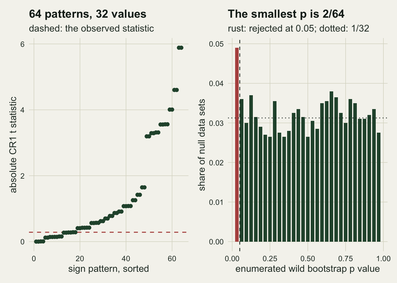
What six catchments can detect
Holding the level is half the job. The same seven procedures, applied to six-catchment data sets with a real fence effect of 0.6, the same size as the catchment standard deviation:
beta_alt <- 0.6; n_pow <- 2000
set.seed(66006)
pow_out <- vapply(seq_len(n_pow), function(i) run_set(6, beta = beta_alt), numeric(14))
pow <- rowMeans(pow_out[meth_key, ])
mcse_pow <- sqrt(max(pow * (1 - pow)) / n_pow)
p_wild_alt <- pow_out["p_wild", ]
share_floor_alt <- mean(abs(p_wild_alt - p_floor6) < 1e-9)
set.seed(66007)
pow_means_rows <- vapply(seq_len(n_pow), function(i) {
  d <- gen_catch(6, beta_alt)
  t.test(d$site_mean[d$fenced == 1], d$site_mean[d$fenced == 0], var.equal = TRUE)$p.value
}, 0)
pow_means_01 <- mean(pow_means_rows < 0.01)
pow_diff <- pow["wild"] - pow["means"]
mcse_diff <- sd(pow_out["wild", ] - pow_out["means", ]) / sqrt(n_pow)
Over 2000 data sets the site-means t test detects the effect 0.141 of the time and the wild bootstrap 0.148, with a Monte Carlo standard error of at most 0.011 for any single rate. On the same data sets the difference between those two is +0.007 with a standard error of 0.005, 1.5 standard errors, which this simulation cannot separate from zero. The CR1 against t(5) reaches 0.203, the pairs bootstrap 0.349 and CR1 against the normal 0.324, but those three buy their extra detections with a false alarm rate well above five per cent, so the comparison is not a fair one. The studentised pairs bootstrap detects the effect 0.021 of the time. At one per cent the site-means test still detects it in 0.034 of an independent set of data sets, where the wild bootstrap cannot reject at all.
The more useful number is the low one. An effect as large as the whole catchment standard deviation is detected in a minority of six-catchment studies by the only procedures that hold their level. That is the design, not the analysis; it is what “the unit that counts is the catchment” costs, and no reference distribution rebuilt from the same six numbers can make it cheaper.
If the six catchments go into a mixed model
Many analyses of a design like this never compute catchment means. They fit subplot growth on the fence with a random intercept for catchment, which is the right model, and read the fence coefficient off whatever the package prints. Split-plot designs in ecology shows that in a balanced design the whole-plot test of the full analysis is exactly the analysis of the whole-plot means. The fence here is a whole-plot factor, so the mixed model’s estimate is the same difference of arm means as above, and what is left to decide is its standard error and the distribution it is read against. Package defaults decide both.
A balanced design needs no fitting software for this, which keeps the post free of new packages. REML estimates the variance of one catchment mean as the sum of squares of the catchment means around their arm means divided by G-2, which is the site-means test’s own variance, so its standard error is the site-means standard error. Maximum likelihood divides the same sum by G, which multiplies the standard error by the square root of (G-2)/G. If that estimate falls below the within-catchment variance over twelve, the catchment variance is estimated at zero, on its boundary, and the model pools all the subplots. The function below writes those rules out. Outside this post it was checked on a few hundred six-catchment data sets, boundary fits included, against lme4 1.1-35.1 (lmer by REML and by ML), glmmTMB 1.1.8, and emmeans 1.10.0 with pbkrtest 0.5.2: the standard errors agree to the fitting tolerance, and the Kenward-Roger test comes out on G-2 degrees of freedom with the REML standard error.
mm_se <- function(d, reml = TRUE, n = n_plot) {
  G <- d$G; mbar <- d$site_mean
  ss_b <- sum((mbar - ave(mbar, d$fenced))^2)   # catchment means around their arm mean
  v_mean <- ss_b / (if (reml) G - 2 else G)      # variance of one catchment mean
  bnd <- v_mean < d$ss_within / (d$N - G) / n    # catchment variance estimated at zero
  if (bnd) v_mean <- (d$ss_within + n * ss_b) / (if (reml) d$N - 2 else d$N) / n
  c(se = sqrt(v_mean * 4 / G), bnd = bnd, se_means = sqrt(ss_b / (G - 2) * 4 / G))
}
mm_run <- function(G, gen = gen_catch, n = n_plot, n_sets = 4000) {
  vapply(seq_len(n_sets), function(i) {
    d <- gen(G)
    b <- mean(d$site_mean[d$fenced == 1]) - mean(d$site_mean[d$fenced == 0])
    r <- mm_se(d, TRUE, n); m <- mm_se(d, FALSE, n)
    c(reml_z  = abs(b / r[["se"]]) > qnorm(0.975),        # lmer summary read against the normal
      ml_z    = abs(b / m[["se"]]) > qnorm(0.975),        # glmmTMB default: ML and Wald z
      reml_t  = abs(b / r[["se"]]) > qt(0.975, G - 2),    # Kenward-Roger here: G-2 df
      means   = abs(b / r[["se_means"]]) > qt(0.975, G - 2),
      means_z = abs(b / r[["se_means"]]) > qnorm(0.975),
      ml_raw  = abs(b / (r[["se_means"]] * sqrt((G - 2) / G))) > qnorm(0.975),
      bnd     = r[["bnd"]], bnd_ml = m[["bnd"]])
  }, numeric(8))
}
mm_n_big <- 600                                  # the same generator, 600 subplots each
mm_gen_big <- gen_catch
environment(mm_gen_big) <- list2env(list(n_plot = mm_n_big), parent = environment(gen_catch))
set.seed(8450); mm6 <- mm_run(6)
set.seed(8451); mm10 <- mm_run(10)
set.seed(8452); mm_big <- mm_run(6, mm_gen_big, n = mm_n_big)
mm_cf <- function(G) c(reml_z = 2 * pt(-qnorm(0.975), G - 2),
                       ml_z = 2 * pt(-qnorm(0.975) * sqrt((G - 2) / G), G - 2))
mm_r6 <- rowMeans(mm6); mm_r10 <- rowMeans(mm10); mm_rbig <- rowMeans(mm_big)
mm_p <- c(mm_r6[1:6], mm_r10[1:2], mm_rbig[1]); mm_mcse <- sqrt(max(mm_p * (1 - mm_p)) / ncol(mm6))
mm_b6 <- mm6["bnd", ] == 1; mm_cz <- mm_cf(6)[["reml_z"]]   # z: site-means rate vs its closed form
mm_zgap <- (mm_cz - mm_r6[["means_z"]]) / sqrt(mm_cz * (1 - mm_cz) / ncol(mm6))
stopifnot(all(mm6["reml_t", !mm_b6] == mm6["means", !mm_b6]),   # the site-means t test
          all(mm6["reml_z", !mm_b6] == mm6["means_z", !mm_b6]),
          all(mm6["reml_t", ] <= mm6["means", ]),
          all(mm6["reml_z", ] <= mm6["means_z", ]),
          all(mm6["ml_z", ] <= mm6["ml_raw", ]),
          all(mm6["ml_z", mm6["bnd_ml", ] == 0] == mm6["ml_raw", mm6["bnd_ml", ] == 0]), abs(mm_zgap) < 3)
The defaults, checked in the versions installed here (lme4 1.1-35.1, emmeans 1.10.0, glmmTMB 1.1.8), with the three arguments unchanged in the current sources on GitHub (lme4 2.1-0, emmeans 2.0.5, glmmTMB 1.1.15.1): lmer fits by REML (REML = TRUE), and its summary() prints a t value with no degrees of freedom and no p value, so the reader supplies the reference; reading |t| > 1.96 as significant is a normal reference. emmeans computes Kenward-Roger or Satterthwaite degrees of freedom for an lmer fit only while the model has at most 3000 rows (pbkrtest.limit and lmerTest.limit); above that it switches to asymptotic degrees of freedom, which is a z test, and says so in a message that a chunk with message: false never shows. The two degrees-of-freedom methods are not interchangeable here. Checked outside this post with lmerTest 3.1.3, whose summary() prints Satterthwaite degrees of freedom once it is loaded, they agree on G-2 while the catchment variance is estimated above zero, but on a singular fit Satterthwaite gives N-2, 70 in this design, where Kenward-Roger stays on G-2; emmeans uses Kenward-Roger by default. glmmTMB fits by maximum likelihood (REML = FALSE) and its summary reports Wald z.
library(lme4)
fit <- lmer(growth ~ fenced + (1 | catchment), data = subplots)  # REML by default
summary(fit)                               # t value, no df, no p value
library(emmeans)
emm_options(pbkrtest.limit = 1e5, lmerTest.limit = 1e5)  # keep the df above 3000 rows
pairs(emmeans(fit, ~ fenced))              # Kenward-Roger df
library(glmmTMB)
fit_ml <- glmmTMB(growth ~ fenced + (1 | catchment), data = subplots)  # ML by default
summary(fit_ml)                            # Wald z
Over 4000 null data sets at six catchments, the REML standard error read against the normal rejects a true null at 0.108, and the maximum likelihood standard error read against the normal, glmmTMB’s default output, at 0.167. The closed forms in the style of the sandwich section are 2 pt(-1.96, G-2) = 0.122 and 2 pt(-1.96 sqrt((G-2)/G), G-2) = 0.185. The REML standard error read against t on G-2 degrees of freedom, which is what Kenward-Roger gives here, rejects at 0.041, next to 0.050 for the site-means t test on the same data sets. No rate in this section taken over all 4000 data sets of a cell has a Monte Carlo standard error above 0.0061.
The closed forms describe the site-means standard error, and the model uses it only while the catchment variance is estimated above zero. By REML it is estimated at zero in 0.056 of these data sets, and those are the data sets whose catchment means sit closest to their arm means, so the site-means standard error there is small; the model replaces it with a larger pooled one. On those 224 fits the normal reference rejects at 0.411 with the model’s standard error and would reject at 0.518 with the site-means one. Across all the data sets the site-means standard error against the normal rejects at 0.115, 1.4 Monte Carlo standard errors below its closed form of 0.122, which it matches in expectation because the site-means statistic is exactly t on G-2 (the chunk stops if the gap exceeds three). The whole gap to the model’s 0.108 comes from the boundary fits. Maximum likelihood reaches the boundary more often, in 0.112 of the data sets; its unpooled standard error against the normal rejects at 0.180, and again the gap to the model’s 0.167 is the boundary fits. Away from the boundary the REML test on G-2 degrees of freedom is the site-means t test, decision for decision (the chunk stops if not), and on the boundary it can only reject less often. At ten catchments the two normal-reference rates are 0.084 and 0.113, against closed forms of 0.086 and 0.118, with 0.009 of fits on the boundary.
The row-count switch is the default that changes the answer without changing anything the analyst typed. This design has 72 rows, far below 3000. The same six catchments with 600 subplot readings each, a logger grid rather than twelve quadrats, have 3600 rows, and emmeans then reads the REML statistic against the normal. On 4000 such data sets that rejects at 0.122, against the unchanged closed form of 0.122: the subplot count does not enter it, and with that many readings none of the fits reach the boundary. The extra subplots do not help: they remove the boundary fits, and the normal reference then over-rejects by the full closed-form amount. Raising the two limits restores the G-2 degrees of freedom. All of this is for the balanced design of this post, where Kenward-Roger reduces to the site-means test; how close it stays in an unbalanced design was not measured here.
What to report
Say how many catchments there were, and how many were treated, before any test statistic. At six with three treated, that count decides which tests hold their level; the number of subplots does not enter the degrees of freedom of the site-means test at all.
For a balanced design with a treatment constant inside each catchment, report the site-means analysis as the primary one: the difference between arm means of the catchment means, its standard error, and its t interval on G-2 degrees of freedom. At six catchments that is six numbers and one call to t.test, it is exact under normal catchment effects, and it held its level here at every catchment count. Donald and Lang 2007 give the general version for group-level regressors.
If the design is unbalanced enough that the site means are not a clean analysis (unequal subplot counts, covariates that vary inside catchments), a wild cluster bootstrap with the null imposed is the next step, and its p value should be printed with its floor: at G catchments with signs of plus or minus the smallest attainable two-sided p is 2/2^G. A p value of 0.0312 from six catchments is the most extreme result the method can produce, not a strong result.
Do not report a pairs cluster bootstrap interval or a CR1 standard error against a normal reference at single-digit catchment counts. If the CR1 sandwich is used at all, it goes against t(G-1) with the reminder that a between-catchment treatment makes even that liberal. If the analysis is a mixed model, fit it by REML, read the fence effect on G-2 degrees of freedom, and check that the software has not switched to a normal reference. If a pairs bootstrap is used, report the share of degenerate resamples and how they were handled.
Honest limits
Everything here is balanced: equal subplot counts, half the catchments treated, normal catchment effects with a common variance. That is the setting in which the site-means test is exact and the sandwich has a closed form, and it is also the most favourable setting for the wild bootstrap. MacKinnon and Webb 2017 show that when cluster sizes differ a lot the sandwich t test over-rejects even with fifty clusters while the wild cluster bootstrap copes, but that the wild bootstrap itself stops holding its level when only one or two clusters are treated. A paired design with one impact catchment and five controls is outside what was measured here, and the one-impact-site design itself is introduced in Before-after-control-impact designs.
The site-means test is exact only under normal catchment effects with equal variance in the two arms. A strongly skewed response, or a fence that changes the between-catchment variance as well as the mean, weakens it, and with three catchments per arm there is too little information to check either assumption from the data. A permutation test on the six means is the assumption-light alternative, but with three of six treated it has only 20 arrangements, and each arrangement and its swap give the same absolute difference, so its smallest two-sided p value is 0.10: it cannot reject at five per cent at all.
The pairs bootstrap was taken as percentile and studentised forms with 499 resamples. Other variants exist (bias-corrected intervals, stratified resampling within arms), and a pairs bootstrap stratified by treatment arm would never produce a degenerate resample. Stratification does not remove the variance shrinkage, but it was not measured here.
The studentised pairs bootstrap’s collapse comes from resamples with one arm made of a single repeated catchment (0.420 of draws). Only 0.012 of draws have both arms like that and a sandwich variance of zero, and in the simulation they make up 0.012 of the resamples that have a slope. The rule used here counts those as infinitely extreme. Dropping them instead can only lower the critical value, and at six catchments it barely moves the rejection rate: 0.007 [0.007, 0.007] against 0.007 [0.003, 0.007] with them counted.
The reproduction of the bootstrap post’s arm used its design and its percentile interval but a vectorised resampler rather than its loop. The two are the same procedure; that post’s own coverage chunk, rerun separately for this post, falls inside the five-block range at twenty sites, but its single run and the blocks here use different seeds.
References
Hurlbert SH 1984 Ecological Monographs 54(2):187-211 (10.2307/1942661)
Cameron AC, Gelbach JB, Miller DL 2008 Review of Economics and Statistics 90(3):414-427 (10.1162/rest.90.3.414)
MacKinnon JG, Webb MD 2017 Journal of Applied Econometrics 32(2):233-254 (10.1002/jae.2508)
Donald SG, Lang K 2007 Review of Economics and Statistics 89(2):221-233 (10.1162/rest.89.2.221)