library(ggplot2)

te_pal <- list(forest = "#275139", green = "#2f8f63", sage = "#93a87f",
               clay = "#b5534e", gold = "#cda23f", line = "#dad9ca",
               ink = "#16241d", paper = "#f5f4ee")

theme_te <- function() {
  theme_minimal(base_size = 12) +
    theme(panel.grid.minor = element_blank(),
          panel.grid.major = element_line(colour = "#e7e6dc"),
          plot.background = element_rect(fill = "#f5f4ee", colour = NA),
          panel.background = element_rect(fill = "#f5f4ee", colour = NA),
          plot.title = element_text(face = "bold", colour = te_pal$ink),
          axis.title = element_text(colour = "#2c3a31"),
          axis.text = element_text(colour = "#2c3a31"))
}Dependent effect sizes in meta-analysis
R
meta-analysis
effect size
heterogeneity
ecology tutorial
Most studies report several effect sizes, so they are not independent. A simulation prices the naive pooled fit, the three-level model and clustered errors.
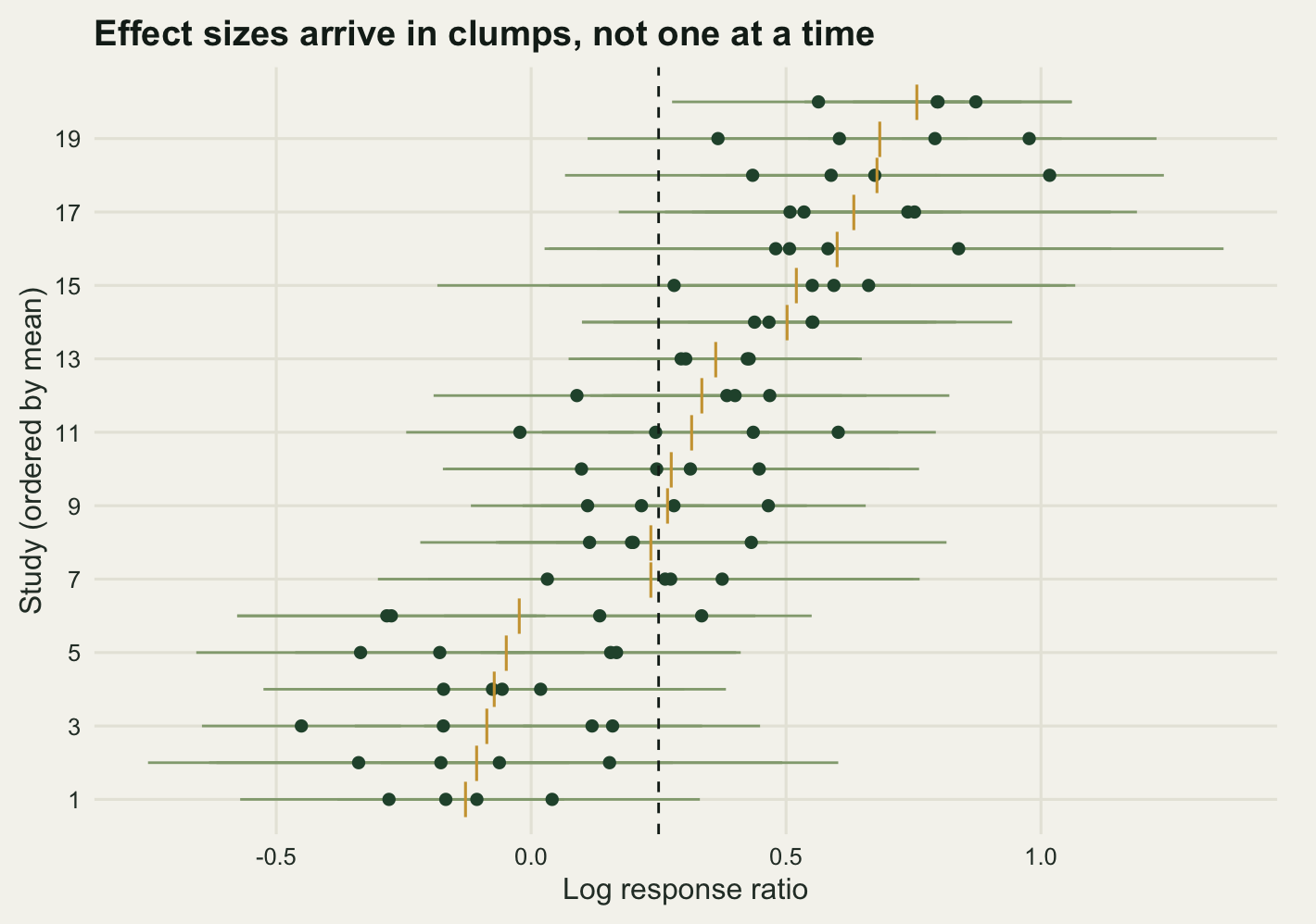
A synthesis of warming experiments on plant growth: twenty published studies, open-top chambers or buried heating cables, one to five growing seasons, aboveground biomass in warmed plots against ambient controls. The effect metric is the log response ratio, and almost none of the studies reports one of them. A chamber experiment that measured four species reports four ratios. A study with two response variables at two sites reports four. Twenty studies, eighty effect sizes, and the spreadsheet that comes out of the literature search has eighty rows.
Fitting a random-effects model to those eighty rows is a single line of code and it is the default in every meta-analysis package. It also assumes that the eighty rows are eighty independent draws. They are not. Four ratios from one chamber experiment share a site, a climate, a soil, a warming magnitude, an observer, and often the same plants: whatever made that experiment’s response large or small applies to all four. The rows arrive in clumps and the model treats them as if they had arrived one at a time.
This is the point at which random-effects meta-analysis in R stops. That post builds the two-level model and says in its limits that the model assumes the studies are independent, and that multiple effects from one study break the assumption and call for a multilevel meta-analysis. This is that continuation. Heterogeneity in meta-analysis owns tau-squared, Cochran’s Q and I-squared, and works entirely inside the independent case; the last section here is about what happens to all three once the effect sizes come in clumps.
The error is the same shape as pseudoreplication one level down, and the difference is worth naming because it changes what the fix can be. In a primary dataset the fish inside a tank are raw measurements, and if you distrust the model you can fall back on the tank means and analyse eight numbers. In a meta-analysis the raw data are gone. What survives is an effect size and a sampling variance treated as known, computed from sample sizes and standard deviations printed in a table. The dependence lives in the effect sizes themselves, and the variances that describe their precision are inputs rather than things the fit estimates. That constrains every repair below.
Pappalardo, Song, Hungate and Osenberg re-examined ninety-six global-change meta-analyses in 2023 and found that sixty-six per cent acknowledged some form of non-independence, leaving about a third that never raised it, and that sixteen per cent went as far as modelling one of its sources. Most of the rest chose one effect per study or averaged them, which are both defensible, and one of them turns out below to be harder than it looks.
This post simulates that spreadsheet and measures five things: how far the naive interval falls short, how many independent effect sizes eighty clumped ones are actually worth, what each of the three standard repairs costs in width and buys in coverage, where the averaging repair breaks in a way its coverage does not reveal, and what tau-squared and I-squared mean once the variance is split across two levels.
Two ways an effect size can be tied to its neighbours
Write \(y_{ij}\) for the \(j\)th effect size in study \(i\), \(\theta_{ij}\) for the true effect it estimates, and \(v_{ij}\) for its sampling variance, known. The generating model has three layers:
\[y_{ij} = \mu + u_i + w_{ij} + \varepsilon_{ij}, \qquad u_i \sim N(0, \tau^2_b), \quad w_{ij} \sim N(0, \tau^2_w)\]
\(u_i\) is what the study contributes to all of its effects: the site, the warming magnitude, the season length. \(w_{ij}\) is what separates one species or one response variable from another inside the same study. Together they say the true effects come in clumps, and their ratio \(\tau^2_b/(\tau^2_b + \tau^2_w)\) is the share of the heterogeneity that lives between studies rather than inside them.
The second tie is in the sampling error. If a study reports biomass and height for the same plants, the two effect sizes come from overlapping measurements and their sampling errors are correlated even though each variance is reported separately. Write \(\mathrm{cov}(\varepsilon_{ij}, \varepsilon_{il}) = r\sqrt{v_{ij}v_{il}}\) for \(j \neq l\), with \(r\) the sampling correlation, and zero across studies. Nothing in a published table tells you what \(r\) is, which is the whole reason the third repair below exists. What matters for everything that follows is the correlation between two observed effect sizes from the same study,
\[\rho = \frac{\tau^2_b + r\sqrt{v_{ij}v_{il}}} {\sqrt{(\tau^2_b + \tau^2_w + v_{ij})(\tau^2_b + \tau^2_w + v_{il})}}\]
which mixes both ties into one number. The simulation is tuned so that \(\rho\) averages about 0.6 across the eighty effects.
k_study <- 20
m_eff <- 4
n_es <- k_study * m_eff
mu_true <- 0.25
tau2_b_true <- 0.065
tau2_w_true <- 0.020
r_samp <- 0.25

sim_batch <- function(k, m, tb, tw, rs) {
  n_arm <- sample(5:30, k, replace = TRUE)          # replicate plots per arm
  cv_j <- runif(k * m, 0.30, 0.60)                  # coefficient of variation
  vv <- 2 * cv_j^2 / rep(n_arm, each = m)           # sampling variance of lnRR
  u_i <- rnorm(k, 0, sqrt(tb))                      # study level
  w_ij <- rnorm(k * m, 0, sqrt(tw))                 # effect within study
  a_i <- rnorm(k)                                   # shared sampling noise
  b_ij <- rnorm(k * m)                              # private sampling noise
  e_ij <- sqrt(vv) * (sqrt(rs) * rep(a_i, each = m) + sqrt(1 - rs) * b_ij)
  list(y = mu_true + rep(u_i, each = m) + w_ij + e_ij,
       vv = vv,
       theta = mu_true + rep(u_i, each = m) + w_ij,
       study = rep(seq_len(k), each = m))
}

set.seed(20260801)
one_set <- sim_batch(k_study, m_eff, tau2_b_true, tau2_w_true, r_samp)
rho_set <- mean((tau2_b_true + r_samp * one_set$vv) /
                  (tau2_b_true + tau2_w_true + one_set$vv))

print(round(c(studies = k_study, effects_per_study = m_eff, effect_sizes = n_es,
              true_mean = mu_true, tau2_between = tau2_b_true, tau2_within = tau2_w_true,
              sampling_correlation = r_samp, median_v = median(one_set$vv),
              mean_rho = rho_set), 4))
studies effects_per_study effect_sizes
20.0000 4.0000 80.0000
true_mean tau2_between tau2_within
0.2500 0.0650 0.0200
sampling_correlation median_v mean_rho
0.2500 0.0210 0.6482 The dataset holds 80 effect sizes from 20 studies, 4 each, with a true pooled log response ratio of 0.25 (about a 28.4 per cent increase in biomass), a median sampling variance of 0.021, and an average within-study correlation of 0.648. Of the total heterogeneity, 76.5 per cent sits between studies and the rest inside them.
Writing both fits out
The three-level model has a marginal covariance that is block diagonal, with one block per study. For a study with \(m\) effects,
\[\Sigma_i = \tau^2_b \mathbf{1}\mathbf{1}^{\top} + D_i, \qquad D_i = \mathrm{diag}(\tau^2_w + v_{ij})\]
and the naive model is the same thing with \(\tau^2_b\) set to zero, which is why one function covers both. Inverting a block by brute force would be wasteful: \(\Sigma_i\) is a diagonal matrix plus a rank-one term, so the Sherman-Morrison identity gives the inverse in closed form,
\[\Sigma_i^{-1} = D_i^{-1} - \frac{\tau^2_b\, D_i^{-1}\mathbf{1}\mathbf{1}^{\top}D_i^{-1}} {1 + \tau^2_b\, \mathbf{1}^{\top}D_i^{-1}\mathbf{1}}\]
Because the only covariate is an intercept, every quantity the fit needs collapses to two sums per study. Write \(s_i = \sum_j 1/(\tau^2_w + v_{ij})\) and \(t_i = \sum_j y_{ij}/(\tau^2_w + v_{ij})\). Then
\[\mathbf{1}^{\top}\Sigma_i^{-1}\mathbf{1} = \frac{s_i}{1 + \tau^2_b s_i}, \qquad \mathbf{1}^{\top}\Sigma_i^{-1}y_i = \frac{t_i}{1 + \tau^2_b s_i}, \qquad \log|\Sigma_i| = \sum_j \log(\tau^2_w + v_{ij}) + \log(1 + \tau^2_b s_i)\]
so the generalised least squares mean and its variance are
\[\hat\mu = \frac{\sum_i t_i/(1 + \tau^2_b s_i)}{\sum_i s_i/(1 + \tau^2_b s_i)}, \qquad \mathrm{Var}(\hat\mu) = \Big(\sum_i \frac{s_i}{1 + \tau^2_b s_i}\Big)^{-1}\]
Both variance components come out of restricted maximum likelihood, which is what meta-analysis software reports by default and which corrects the downward bias that plain maximum likelihood puts on \(\tau^2\). The restricted log-likelihood is the usual one for a linear model with known error variances. Konstantopoulos worked through the fixed-effect and variance-component estimation for this model in 2011, and Cheung showed in 2014 that the same fit can be obtained as a structural equation model, which is why the three-level meta-analysis turns up under two different names in the applied literature.
blk <- function(x, m) colSums(matrix(x, nrow = m))

ll_reml <- function(tb, tw, y, vv, m) {
  dv <- tw + vv
  s_i <- blk(1 / dv, m)
  t_i <- blk(y / dv, m)
  den <- 1 + tb * s_i
  info <- sum(s_i / den)
  mu <- sum(t_i / den) / info
  ev <- y - mu
  te <- blk(ev / dv, m)
  quad <- sum(ev^2 / dv) - tb * sum(te^2 / den)
  list(ll = -0.5 * (sum(log(dv)) + sum(log(den)) + log(info) + quad),
       mu = mu, se = sqrt(1 / info))
}

fit_re <- function(y, vv) {                       # naive two-level fit
  op <- optimize(function(tw) -ll_reml(0, tw, y, vv, 1)$ll, c(0, 3), tol = 1e-9)
  rr <- ll_reml(0, op$minimum, y, vv, 1)
  c(mu = rr$mu, se = rr$se, tau2 = op$minimum)
}

fit_3l <- function(y, vv, m) {                    # effects within studies
  op <- optim(c(0.05, 0.02), function(p) -ll_reml(p[1], p[2], y, vv, m)$ll,
              method = "L-BFGS-B", lower = c(0, 0), upper = c(3, 3))
  rr <- ll_reml(op$par[1], op$par[2], y, vv, m)
  c(mu = rr$mu, se = rr$se, tau2_b = op$par[1], tau2_w = op$par[2])
}

naive_one <- fit_re(one_set$y, one_set$vv)
three_one <- fit_3l(one_set$y, one_set$vv, m_eff)

print(round(naive_one, 5))
mu se tau2
0.29514 0.03809 0.09110 print(round(three_one, 5)) mu se tau2_b tau2_w
0.29806 0.06660 0.07730 0.02064 On this one dataset the naive fit returns a pooled effect of 0.2951 with a standard error of 0.0381, and the three-level fit returns 0.2981 with a standard error of 0.0666, a factor of 1.75 wider. The point estimates barely move, which is the first thing to hold on to: clustering is not a bias problem. Both fits are aiming at the same \(\mu\) and both hit it. What differs is the claim each one makes about how well it knows the answer.
The naive fit also puts the whole heterogeneity in one number, 0.0911, while the three-level fit splits it into 0.0773 between studies and 0.0206 inside them.
Coverage over two thousand replicates
One dataset settles nothing. The experiment below redraws studies, effects, sampling variances and both kinds of correlated noise two thousand times, and fits five analyses to each replicate: the naive random-effects model on all eighty rows, the study averages with their sampling variance computed the easy way and the correct way, the three-level model, and cluster-robust standard errors applied to the naive fit. The last three get a section each below; here they are only being scored.
fit_crve <- function(y, vv, m, tau2) {            # standard errors clustered by study
  wt <- 1 / (tau2 + vv)
  mu <- sum(wt * y) / sum(wt)
  g_i <- blk(wt * (y - mu), m)
  kk <- length(g_i)
  c(mu = mu, se = sqrt(sum(g_i^2) / sum(wt)^2 * kk / (kk - 1)))
}

agg_var <- function(vmat, rr) {                   # sampling variance of a study mean
  m <- nrow(vmat)
  (colSums(vmat) + rr * (colSums(sqrt(vmat))^2 - colSums(vmat))) / m^2
}

fit_agg <- function(y, vv, m, rr) {
  fit_re(colMeans(matrix(y, nrow = m)), agg_var(matrix(vv, nrow = m), rr))
}set.seed(20260804)
n_rep <- 2000
res <- matrix(NA_real_, n_rep, 14)
for (r in seq_len(n_rep)) {
d <- sim_batch(k_study, m_eff, tau2_b_true, tau2_w_true, r_samp)
fn <- fit_re(d$y, d$vv)
f3 <- fit_3l(d$y, d$vv, m_eff)
fc <- fit_crve(d$y, d$vv, m_eff, fn["tau2"])
fa <- fit_agg(d$y, d$vv, m_eff, r_samp)
fw <- fit_agg(d$y, d$vv, m_eff, 0)
res[r, ] <- c(fn, f3, fc, fa[1:2], fw[1:2],
mean((tau2_b_true + r_samp * d$vv) /
(tau2_b_true + tau2_w_true + d$vv)))
}
colnames(res) <- c("mu_n", "se_n", "t2_n", "mu_3", "se_3", "tb_3", "tw_3",
"mu_c", "se_c", "mu_a", "se_a", "mu_w", "se_w", "rho")
res <- as.data.frame(res)
z95 <- qnorm(0.975)
t95 <- qt(0.975, k_study - 1)
cvg <- function(mu, se, crit) 100 * mean(abs(mu - mu_true) < crit * se)
rho_bar <- mean(res$rho)
cov_naive <- cvg(res$mu_n, res$se_n, z95)
cov_3l <- cvg(res$mu_3, res$se_3, z95)
cov_3l_t <- cvg(res$mu_3, res$se_3, t95)
cov_crve <- cvg(res$mu_c, res$se_c, t95)
cov_agg <- cvg(res$mu_a, res$se_a, t95)
cov_aggw <- cvg(res$mu_w, res$se_w, t95)
se_short <- 100 * (1 - mean(res$se_n) / sd(res$mu_n))
width_ratio <- mean(res$se_3) / mean(res$se_n)
mc_se <- 100 * sqrt(0.95 * 0.05 / n_rep)
print(round(c(mean_rho = rho_bar, replicates = n_rep, sd_of_estimate = sd(res$mu_n),
bias_naive = mean(res$mu_n) - mu_true, bias_three = mean(res$mu_3) - mu_true,
mean_se_naive = mean(res$se_n), mean_se_three = mean(res$se_3),
se_shortfall_pct = se_short), 5)) mean_rho replicates sd_of_estimate bias_naive
0.63876 2000.00000 0.06451 0.00060
bias_three mean_se_naive mean_se_three se_shortfall_pct
0.00054 0.03668 0.06302 43.14081 print(round(c(coverage_naive = cov_naive, coverage_three_z = cov_3l,
coverage_three_t = cov_3l_t, coverage_clustered = cov_crve,
coverage_average_correct = cov_agg, coverage_average_easy = cov_aggw,
monte_carlo_se = mc_se), 3)) coverage_naive coverage_three_z coverage_three_t
73.250 93.300 94.800
coverage_clustered coverage_average_correct coverage_average_easy
94.450 94.550 94.850
monte_carlo_se
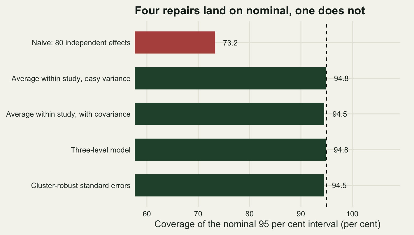
0.487 Over 2000 replicates the naive interval covers the true pooled effect 73.25 per cent of the time against a nominal 95, and the reason is in the line above it: the standard deviation of the naive estimate across replicates is 0.0645 while the standard error it reports averages 0.0367. The fit understates its own uncertainty by 43.1 per cent. Both estimators are essentially unbiased, the naive one by 0.00060 and the three-level one by 0.00054, so nothing is wrong with the number in the middle of the interval. Only the interval is wrong.
The three-level model brings coverage back to 93.3 per cent against a normal reference and 94.8 per cent against a \(t\) reference on 19 degrees of freedom, the fairer comparison once you accept that the pooled mean is an average over 20 studies rather than 80 effects. The Monte Carlo standard error on a percentage near nominal is 0.49, so the four analyses scored in the figure below are indistinguishable from nominal and from each other, and the naive one is 45 of those Monte Carlo standard errors away. The three-level fit read against a normal reference is the one exception, 3.5 standard errors short, which is the price of pretending the pooled mean rests on 80 effects rather than 20 studies.
The price is the width. The three-level standard error averages 0.063 against the naive 0.0367, a factor of 1.718. The naive analysis reports an interval 41.8 per cent narrower than the evidence supports, so correcting it means publishing a synthesis that looks 1.72 times less decisive than the one the default code produced.
How many studies is eighty effect sizes worth
The naive fit is confident because it counts eighty pieces of evidence. The arithmetic that says how many there really are is the design effect, the same formula that governs cluster sampling. At equal weights and equal marginal variances \(\sigma^2\) the naive fit believes \(\mathrm{Var}(\hat\mu) = \sigma^2/km\), while the truth adds one covariance term for each of the \(m(m-1)\) ordered pairs inside each study:
\[\mathrm{Var}(\hat\mu) = \frac{1}{(km)^2}\Big(km\,\sigma^2 + km(m-1)\rho\,\sigma^2\Big) = \frac{\sigma^2}{km}\big(1 + (m-1)\rho\big)\]
The bracket is the design effect. Dividing the number of effect sizes by it gives the effective number of independent effect sizes: the count of one-effect studies that would deliver the same precision.
de_meas <- (sd(res$mu_n) / mean(res$se_n))^2
de_pred <- 1 + (m_eff - 1) * rho_bar
n_eff_meas <- n_es / de_meas
n_eff_pred <- n_es / de_pred
rho_grid <- seq(0, 1, by = 0.01)
n_eff_curve <- n_es / (1 + (m_eff - 1) * rho_grid)

print(round(c(design_effect_measured = de_meas, design_effect_predicted = de_pred,
              effective_effects_measured = n_eff_meas, effective_effects_predicted = n_eff_pred,
              floor_at_rho_one = n_es / m_eff, nominal_effects = n_es), 4))
design_effect_measured design_effect_predicted
3.0931 2.9163
effective_effects_measured effective_effects_predicted
25.8637 27.4321
floor_at_rho_one nominal_effects
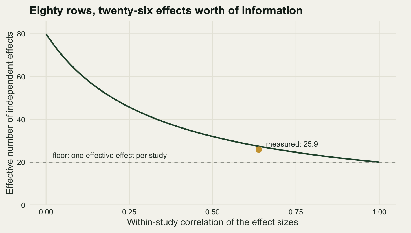
20.0000 80.0000 The measured design effect is 3.093, against 2.916 from the formula at the average correlation of 0.639. The two differ because the fit uses inverse-variance weights rather than equal ones and the sampling variances are not equal, but the formula is close enough to use as a back of the envelope check on a real synthesis.
So the eighty effect sizes carry the information of about 25.9 independent ones. The lower bound is worth seeing: as \(\rho\) goes to one the design effect goes to \(m\), the effective count goes to \(km/m = k\), and eighty effect sizes collapse to 20, the number of studies. At 0.64 the count sits at 25.9, which is much nearer the twenty-study floor than the eighty-row claim on the spreadsheet. That is the sentence to carry into a synthesis: adding a fifth species to a study that already reports four adds very little, and adding a twenty-first study adds a great deal.
Averaging within a study is a covariance calculation
The oldest repair is to reduce each study to one number and pool the twenty. It is honest, it needs no new machinery, and it is what most of the meta-analyses in the Pappalardo survey did. The trap is in the second step, because collapsing a study to its mean means you now have to say what the sampling variance of that mean is, and the answer is not the mean of the sampling variances. Lajeunesse set out the algebra for response ratios in 2011, for the two designs that produce it most often in ecology: several outcomes measured on one set of plants, and several treatment arms compared against one shared control.
For a study with \(m\) effects and sampling covariance matrix \(V_i\),
\[\mathrm{Var}(\bar{y}_i) = \frac{1}{m^2}\mathbf{1}^{\top}V_i\mathbf{1} = \frac{1}{m^2}\Big(\sum_j v_{ij} + \sum_{j \neq l} r\sqrt{v_{ij}v_{il}}\Big)\]
The first sum is what you get by assuming the effects are independent. The second is the correction, it has \(m(m-1)\) terms against the first sum’s \(m\), and it is zero only if the sampling errors really are uncorrelated. With four effects of equal variance \(v\) and a sampling correlation of 0.25, the correct variance is \((4v + 3v)/16 = 0.4375v\) against the easy answer of \(0.25v\), larger by three quarters.
set.seed(70101)
n_rep_a <- 3000
hit_c <- hit_w <- 0
n_seen <- 0
ratio_acc <- 0
for (r in seq_len(n_rep_a)) {
  d <- sim_batch(k_study, m_eff, tau2_b_true, tau2_w_true, r_samp)
  vmat <- matrix(d$vv, nrow = m_eff)
  ybar <- colMeans(matrix(d$y, nrow = m_eff))
  tbar <- colMeans(matrix(d$theta, nrow = m_eff))
  v_ok <- agg_var(vmat, r_samp)
  v_easy <- agg_var(vmat, 0)
  hit_c <- hit_c + sum(abs(ybar - tbar) < z95 * sqrt(v_ok))
  hit_w <- hit_w + sum(abs(ybar - tbar) < z95 * sqrt(v_easy))
  ratio_acc <- ratio_acc + mean(sqrt(v_ok / v_easy))
  n_seen <- n_seen + k_study
}
cov_study_ok <- 100 * hit_c / n_seen
cov_study_easy <- 100 * hit_w / n_seen
se_ratio_agg <- ratio_acc / n_rep_a

print(round(c(study_intervals = n_seen, coverage_with_covariance = cov_study_ok,
              coverage_easy_way = cov_study_easy, se_ratio = se_ratio_agg,
              se_shortfall_pct = 100 * (1 - 1 / se_ratio_agg)), 4))
study_intervals coverage_with_covariance coverage_easy_way
60000.0000 95.0517 86.4417
se_ratio se_shortfall_pct
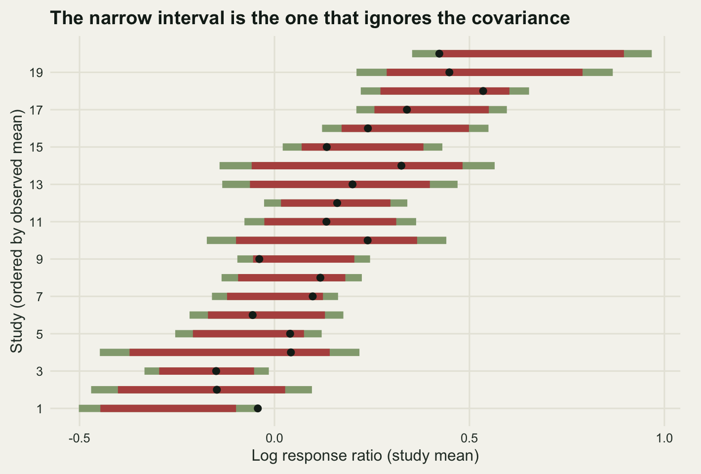
1.3126 23.8125 Scored on the quantity it actually claims, the easy answer fails. Across 60,000 study-level intervals from 3000 replicates, the interval built from the correct sampling variance covers the study’s own mean true effect 95.05 per cent of the time, and the interval built by summing the variances alone covers it 86.44 per cent of the time. The standard error is a factor of 1.313 too small, which is 23.8 per cent short. Those are the intervals a forest plot draws, and they are the weights a precision-weighted pool uses.
The pooled mean is a different story, and this went against what I expected before running it.
set.seed(70102)
n_rep_t <- 1500
acc_ok <- acc_easy <- 0
for (r in seq_len(n_rep_t)) {
  d <- sim_batch(k_study, m_eff, tau2_b_true, tau2_w_true, r_samp)
  acc_ok <- acc_ok + fit_agg(d$y, d$vv, m_eff, r_samp)["tau2"]
  acc_easy <- acc_easy + fit_agg(d$y, d$vv, m_eff, 0)["tau2"]
}
t2_ok <- unname(acc_ok / n_rep_t)
t2_easy <- unname(acc_easy / n_rep_t)
t2_target <- tau2_b_true + tau2_w_true / m_eff

print(round(c(tau2_of_study_means_true = t2_target, tau2_with_covariance = t2_ok,
              tau2_easy_way = t2_easy, inflation_pct = 100 * (t2_easy / t2_ok - 1),
              coverage_pooled_with_covariance = cov_agg,
              coverage_pooled_easy_way = cov_aggw), 5))
tau2_of_study_means_true tau2_with_covariance
0.07000 0.07066
tau2_easy_way inflation_pct
0.07598 7.51989
coverage_pooled_with_covariance coverage_pooled_easy_way
94.55000 94.85000 Coverage of the pooled mean is 94.55 per cent with the covariance term and 94.85 per cent without it, a gap of 0.3 points against a Monte Carlo standard error of 0.49. The mistake does not show up at all. The reason is that the random-effects fit on the twenty study means estimates \(\tau^2\) from the scatter of those means, and if you hand it sampling variances that are too small it simply calls the difference heterogeneity: \(\tau^2\) comes out at 0.076 instead of 0.0707, an inflation of 7.5 per cent, and the sum of the two that drives the interval barely moves. The true value for the study means is \(\tau^2_b + \tau^2_w/m =\) 0.07, which the correct calculation recovers and the easy one overshoots.
So the covariance derivation is not optional, but the thing it protects is not the headline interval. It protects the per-study intervals, the weights, the prediction interval for a new study, and every sentence you would write about how much the studies disagree. If the only output is a pooled mean and its interval, a synthesis that ignored the covariance got away with it, and it got away with it by silently relabelling sampling noise as ecology.
Cluster-robust standard errors, and how few studies they survive
The third repair gives up on describing the correlation and estimates the variance of the pooled mean from the between-study scatter of the weighted residuals. Keep the naive fit and its weights \(w_{ij} = 1/(\hat\tau^2 + v_{ij})\), and replace its variance by the sandwich
\[V_R = \frac{k}{k-1}\, \frac{\sum_i \big(\sum_{j \in i} w_{ij} e_{ij}\big)^2} {\big(\sum_{ij} w_{ij}\big)^2}, \qquad e_{ij} = y_{ij} - \hat\mu\]
with the interval taken against a \(t\) distribution on \(k-1\) degrees of freedom. Nothing in that expression needs \(r\), or \(\tau^2_b\), or even a correct weighting scheme: it needs only that the studies are independent of each other and that there are enough of them for the outer sum to behave. Hedges, Tipton and Johnson introduced this for meta-regression with dependent effect sizes in 2010, and the small-print is the same as for every sandwich estimator, which is that the outer sum has \(k\) terms and \(k\) in ecology is often small.
set.seed(70104)
kk_grid <- c(8, 12, 20, 40)
n_rep_k <- 1000
tab_k <- data.frame(k = kk_grid, naive = NA_real_, clustered = NA_real_,
                    three_level = NA_real_)
for (j in seq_along(kk_grid)) {
  kk <- kk_grid[j]
  a_n <- a_c <- a_3 <- 0
  crit_k <- qt(0.975, kk - 1)
  for (r in seq_len(n_rep_k)) {
    d <- sim_batch(kk, m_eff, tau2_b_true, tau2_w_true, r_samp)
    fn <- fit_re(d$y, d$vv)
    fc <- fit_crve(d$y, d$vv, m_eff, fn["tau2"])
    f3 <- fit_3l(d$y, d$vv, m_eff)
    a_n <- a_n + (abs(fn[1] - mu_true) < z95 * fn[2])
    a_c <- a_c + (abs(fc[1] - mu_true) < crit_k * fc[2])
    a_3 <- a_3 + (abs(f3[1] - mu_true) < crit_k * f3[2])
  }
  tab_k[j, 2:4] <- 100 * c(a_n, a_c, a_3) / n_rep_k
}
print(tab_k)
k naive clustered three_level
1 8 70.0 94.3 94.6
2 12 71.4 94.3 94.5
3 20 72.8 93.7 93.7
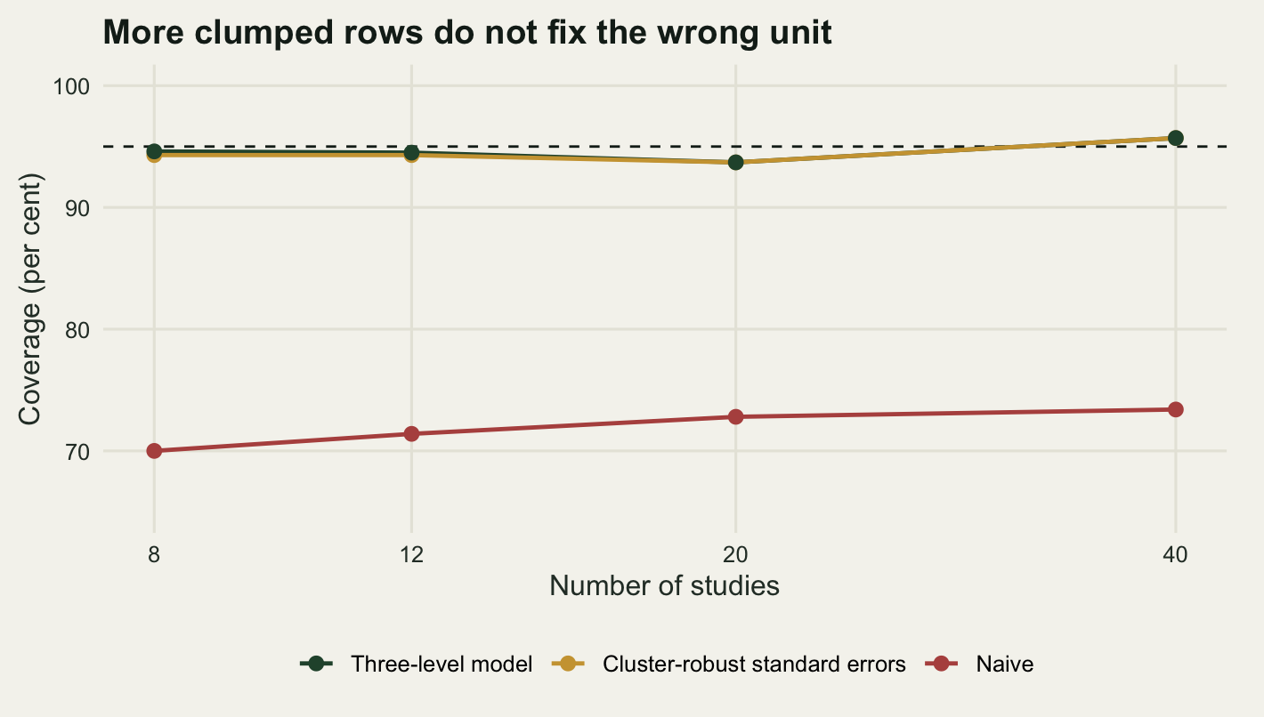
4 40 73.4 95.7 95.7Across 1000 replicates at each study count, the clustered interval holds between 93.7 and 95.7 per cent while the naive one stays between 70 and 73.4 per cent, creeping up by 3.4 points across a fivefold increase in the number of studies rather than moving towards nominal, because its failure is not a small-sample failure. The three-level model tracks the clustered one closely at every count, 94.6 against 94.3 per cent at 8 studies.
That agreement at eight studies is a property of the easiest possible case and should not be generalised. There is one covariate here, an intercept; every cluster has the same size; and the \(t\) reference on 7 degrees of freedom happens to be about right for it. Add a moderator whose values are unbalanced across studies and the effective degrees of freedom fall well below \(k-1\), which is the problem Tipton’s 2015 small-sample corrections exist to solve, and which is why the current advice is to fit the three-level model and put clustered standard errors on top of it rather than choosing between them.
What tau-squared means once it is split
The naive fit reports one \(\tau^2\). The three-level fit reports two, and they are not the two halves of the first one in any simple sense. Start with what each is estimating. The naive \(\tau^2\) describes the marginal variance of a single effect size around the pooled mean, so it targets \(\tau^2_b + \tau^2_w\), the total heterogeneity, and it does so without ever seeing the clustering: the diagonal of the covariance matrix is right in the naive model even though the off-diagonal is missing. The three-level \(\tau^2_b\) describes how much study means differ and \(\tau^2_w\) how much effects differ inside a study.
The experiment below fits the three-level model twice, once to data where the sampling errors within a study are genuinely independent and once to the data used everywhere above, where they correlate at 0.25.
set.seed(70103)
n_rep_s <- 1200
split_indep <- split_corr <- matrix(NA_real_, n_rep_s, 2)
i2_naive <- i2_agg <- i2_between <- i2_within <- numeric(n_rep_s)

typical_v <- function(vv, n_unit) {
  (n_unit - 1) * sum(1 / vv) / (sum(1 / vv)^2 - sum(1 / vv^2))
}

for (r in seq_len(n_rep_s)) {
  d0 <- sim_batch(k_study, m_eff, tau2_b_true, tau2_w_true, 0)
  split_indep[r, ] <- fit_3l(d0$y, d0$vv, m_eff)[3:4]

  d1 <- sim_batch(k_study, m_eff, tau2_b_true, tau2_w_true, r_samp)
  f3 <- fit_3l(d1$y, d1$vv, m_eff)
  split_corr[r, ] <- f3[3:4]

  fn <- fit_re(d1$y, d1$vv)
  vt <- typical_v(d1$vv, n_es)
  i2_naive[r] <- 100 * fn["tau2"] / (fn["tau2"] + vt)
  i2_between[r] <- 100 * f3[3] / (f3[3] + f3[4] + vt)
  i2_within[r] <- 100 * f3[4] / (f3[3] + f3[4] + vt)

  v_a <- agg_var(matrix(d1$vv, nrow = m_eff), r_samp)
  fa <- fit_re(colMeans(matrix(d1$y, nrow = m_eff)), v_a)
  i2_agg[r] <- 100 * fa["tau2"] / (fa["tau2"] + typical_v(v_a, k_study))
}

print(round(c(true_tau2_between = tau2_b_true, true_tau2_within = tau2_w_true,
              indep_tau2_between = mean(split_indep[, 1]),
              indep_tau2_within = mean(split_indep[, 2]),
              corr_tau2_between = mean(split_corr[, 1]),
              corr_tau2_within = mean(split_corr[, 2]),
              naive_tau2_total = mean(res$t2_n),
              true_tau2_total = tau2_b_true + tau2_w_true), 5))
true_tau2_between true_tau2_within indep_tau2_between indep_tau2_within
0.06500 0.02000 0.06542 0.02015
corr_tau2_between corr_tau2_within naive_tau2_total true_tau2_total
0.07054 0.01504 0.08187 0.08500 print(round(c(I2_naive_effect_level = mean(i2_naive), I2_study_level = mean(i2_agg),
I2_between = mean(i2_between), I2_within = mean(i2_within),
I2_three_level_total = mean(i2_between) + mean(i2_within)), 3))I2_naive_effect_level I2_study_level I2_between
78.217 85.532 64.413
I2_within I2_three_level_total
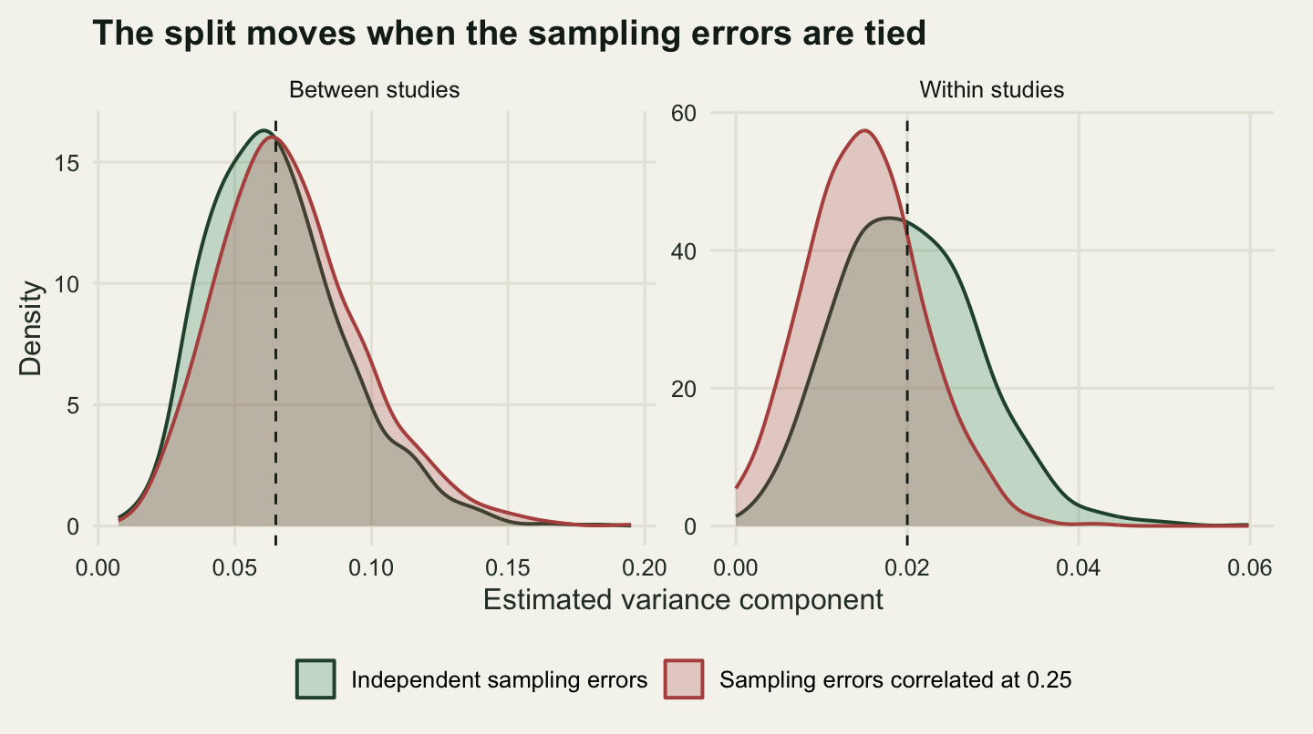
14.681 79.095 With independent sampling errors the split is recovered: 0.0654 and 0.0201 against truths of 0.065 and 0.02. With sampling errors correlated at 0.25 the same fit returns 0.0705 and 0.015: variance has moved from the within level to the between level, by 0.0051 in one direction and 0.0051 in the other, and the total is almost unchanged. In absolute terms the two shifts match; in relative terms they do not, because the same displacement is 7.8 per cent of the between-study component and 25.4 per cent of the smaller within-study one. The mechanism is that a shared sampling error and a shared study effect have the same block structure. If every effect in a study has variance \(v\), then a sampling correlation of \(r\) contributes \(rv\) to every off-diagonal entry of that block, which is algebraically indistinguishable from adding \(rv\) to \(\tau^2_b\) and subtracting it from \(\tau^2_w\). The model cannot tell them apart, so it reports the sum. That is why the coverage was fine and the split was not, and why \(\tau^2_w\) from a three-level fit should be read as a lower bound on true within-study heterogeneity rather than a measurement of it.
I-squared is where the comparability breaks in public. Higgins and Thompson’s definition needs a typical within-study sampling variance, and the answer depends entirely on what a unit is. The same eighty numbers give 78.2 per cent when the unit is the effect size, 85.5 per cent when the unit is the study, and in the three-level fit a between-study share of 64.4 per cent and a within-study share of 14.7 per cent that add to 79.1. None of the three is wrong. They answer three different questions, and a review that lines up I-squared across syntheses which made different choices about the unit is comparing quantities that were never the same. Nakagawa and Santos set out the multilevel version for ecology in 2012, and the practical consequence of their formulation is that an I-squared from a multilevel fit has to be reported with its level attached or not reported at all.
Cochran’s Q inherits the same problem through its degrees of freedom. The naive Q is compared against a chi-squared distribution on 79 degrees of freedom, one per effect size, and the effective count established above is 25.9. A significant Q on eighty clumped effects is not evidence of the same strength as a significant Q on eighty independent ones.
Which one to use
All three repairs landed on nominal and all three cost about the same width. The three-level standard error averaged 0.063, the clustered one 0.063 and the averaged one 0.0633, a spread of 0.37 per cent between the widest and the narrowest. Averaging throws away all the within-study information and still costs almost nothing, which is not a coincidence: at a correlation of 0.64 there was little independent information inside a study to throw away. The choice cannot be made on precision, then, and should be made on what else you want the model to do.
Fit the three-level model when the within-study spread is itself of interest, when moderators vary inside a study (species identity, response variable, year), or when you need a prediction interval that separates the two sources. Use clustered standard errors when you cannot defend a correlation structure and the number of studies is comfortable, which here meant 8 and above for an intercept-only fit and would mean more with moderators. Average within studies when the synthesis genuinely has one question per study, and do the covariance calculation anyway, because the pooled interval survives without it but the forest plot and the heterogeneity statistics do not. The last two combine in practice: fit the three-level model, then cluster the standard errors on top of it, so the structure you can defend does the work and the sandwich covers the part you cannot.
The honest limit
The correlations here were known because I generated them. In a real synthesis \(r\) is not reported and is not estimable from the published summaries either: the covariance between two effect sizes computed on the same plants depends on the correlation between the two response variables in the raw data, which nobody prints. The usual practice is to assume a value, commonly a half, and to check whether the conclusion moves when it is set to zero and to four fifths. The measurements above say what that check will find: the pooled interval will hardly move, because \(\tau^2\) absorbs the difference, while the per-study intervals and the heterogeneity split will move a lot. A sensitivity analysis that reports only the pooled mean looks reassuring for the wrong reason.
The design was balanced, four effects in every study, and real syntheses are not: one study reports one species and another reports eleven. Unbalanced cluster sizes make the effective degrees of freedom for the clustered interval fall below \(k-1\), sometimes far below, and they give the naive fit an extra way to go wrong, because a study with eleven effects gets eleven times the weight of a study with one while contributing barely more independent information. Nothing here measures that, and the correction is Tipton’s, not the plain \(k-1\) used above.
The three-level structure was also the true structure. Real dependence is not always nested: effects can share a research group across studies, a study system, a control group shared by several treatment arms, or a phylogeny, and the last of those needs a correlation matrix rather than a nesting factor. Van den Noortgate and colleagues showed in 2013 that the three-level model handles several of these sources adequately even when it is not literally correct, which is the licence most ecological syntheses are operating under, but the licence runs out when the sharing is not nested at all.
Finally, everything above concerns the interval and not the estimate. Every fit was unbiased for \(\mu\) to within 0.00060. Dependence does not move the pooled effect; it moves the claim about how well you know it, which makes it a quiet error: the number quoted in the abstract is correct and the number that decides whether anyone believes it is not.
Where to go next
The natural next step is a moderator. Once the effects inside a study differ by species or by response variable, the interesting questions become within-study comparisons, and those are estimated more precisely under clustering rather than less, because the study effect cancels in the contrast. That reverses the intuition built above. The second direction is the correlation matrix version: when the dependence is phylogenetic or comes from shared control groups the block is not compound symmetric, the Sherman-Morrison shortcut does not apply, and only the generalised least squares step survives unchanged.
References
Van den Noortgate W, Lopez-Lopez JA, Marin-Martinez F, Sanchez-Meca J 2013 Behavior Research Methods 45(2):576-594 (10.3758/s13428-012-0261-6)
Hedges LV, Tipton E, Johnson MC 2010 Research Synthesis Methods 1(1):39-65 (10.1002/jrsm.5)
Nakagawa S, Santos ESA 2012 Evolutionary Ecology 26(5):1253-1274 (10.1007/s10682-012-9555-5)
Konstantopoulos S 2011 Research Synthesis Methods 2(1):61-76 (10.1002/jrsm.35)
Cheung MWL 2014 Psychological Methods 19(2):211-229 (10.1037/a0032968)
Tipton E 2015 Psychological Methods 20(3):375-393 (10.1037/met0000011)
Higgins JPT, Thompson SG 2002 Statistics in Medicine 21(11):1539-1558 (10.1002/sim.1186)
Lajeunesse MJ 2011 Ecology 92(11):2049-2055 (10.1890/11-0423.1)
Pappalardo P, Song C, Hungate BA, Osenberg CW 2023 PLOS ONE 18(10):e0292606 (10.1371/journal.pone.0292606)