Heterogeneity in meta-analysis

Measure disagreement among ecological studies in base R: Cochran’s Q, I-squared with an interval, tau-squared, and a prediction interval for a new study.

Once a random-effects model tells you the studies disagree, the next question is how much, and in what units. Three quantities are in common use and they answer different questions. Cochran’s Q tests whether there is any excess variation beyond sampling noise. I-squared reports the share of total variation that is between-study. Tau-squared and the prediction interval describe the spread in the units of the effect itself. This post codes all three in base R and shows why I-squared, read on its own, can give a misleading picture of how heterogeneous a body of evidence really is.

A heterogeneous set of studies

We simulate 18 studies of a standardised mean difference, with a true mean effect of 0.35 and a between-study standard deviation of 0.22, so the true tau-squared is 0.0484. As before, each study returns a Hedges’ g and a known sampling variance.

set.seed(201)
mu_true <- 0.35; tau_true <- 0.22; k <- 18
n <- sample(18:130, k, replace = TRUE)

sim_study <- function(theta, ni) {
  x1 <- rnorm(ni, 0, 1); x2 <- rnorm(ni, theta, 1)
  sp <- sqrt(((ni - 1) * sd(x1)^2 + (ni - 1) * sd(x2)^2) / (2 * ni - 2))
  d  <- (mean(x2) - mean(x1)) / sp
  J  <- 1 - 3 / (4 * (2 * ni - 2) - 1)
  g  <- J * d
  vd <- (2 * ni) / (ni * ni) + d^2 / (2 * (2 * ni))
  c(g = g, v = J^2 * vd)
}
theta_i <- rnorm(k, mu_true, tau_true)
gv <- t(mapply(sim_study, theta_i, n))
g  <- gv[, "g"]; v <- gv[, "v"]
wf <- 1 / v; mu_fe <- sum(wf * g) / sum(wf)

Cochran’s Q and I-squared

Q is the inverse-variance weighted sum of squared deviations of each study from the fixed-effect summary. Under the fixed-effect null it follows a chi-squared distribution on k minus one degrees of freedom. I-squared then rescales the excess of Q over its expectation into a proportion.

Q  <- sum(wf * (g - mu_fe)^2)
df <- k - 1
pQ <- pchisq(Q, df, lower.tail = FALSE)
I2 <- max(0, (Q - df) / Q)
c(Q = Q, df = df, p = pQ, I2 = I2)

           Q           df            p           I2 
40.748659079 17.000000000  0.001013717  0.582808358 

Q is 40.7 on 17 degrees of freedom (p = 0.001), and I-squared is 58.3%. A common interval for I-squared is the test-based one of Higgins and Thompson (2002), built from the statistic H equal to the square root of Q over its degrees of freedom.

H   <- sqrt(Q / df)
if (Q > df) {
  se_lnH <- 0.5 * (log(Q) - log(df)) / (sqrt(2 * Q) - sqrt(2 * df - 1))
} else {
  se_lnH <- sqrt(1 / (2 * (df - 1)) * (1 - 1 / (3 * (df - 1)^2)))
}
lnH  <- log(H)
Hlo  <- exp(lnH - 1.96 * se_lnH); Hhi <- exp(lnH + 1.96 * se_lnH)
I2lo <- max(0, (Hlo^2 - 1) / Hlo^2); I2hi <- max(0, (Hhi^2 - 1) / Hhi^2)
c(I2 = I2, lower = I2lo, upper = I2hi)

       I2     lower     upper 
0.5828084 0.2969289 0.7524449 

The interval runs from 29.7% to 75.2%, wide because k is small. Reporting I-squared without its interval hides how little the data pin it down.

Tau-squared with a confidence interval

The between-study variance itself is the DerSimonian-Laird moment estimate. Its interval comes from the Q-profile method (Viechtbauer 2007): the generalised Q, computed at a candidate tau-squared, follows a chi-squared distribution on k minus one degrees of freedom at the true value, so inverting that relationship with uniroot bounds tau-squared.

Cc   <- sum(wf) - sum(wf^2) / sum(wf)
tau2 <- max(0, (Q - df) / Cc)
Qgen <- function(t2) { wi <- 1 / (v + t2); mh <- sum(wi * g) / sum(wi); sum(wi * (g - mh)^2) }
lo_t <- tryCatch(uniroot(function(t2) Qgen(t2) - qchisq(.975, df), c(0, 10))$root,
                 error = function(e) 0)
hi_t <- uniroot(function(t2) Qgen(t2) - qchisq(.025, df), c(0, 10))$root
c(tau2 = tau2, lower = lo_t, upper = hi_t)

      tau2      lower      upper 
0.04470445 0.01254051 0.17352683 

The estimate is 0.045 with an interval from 0.013 to 0.174, and it brackets the true 0.0484.

The prediction interval

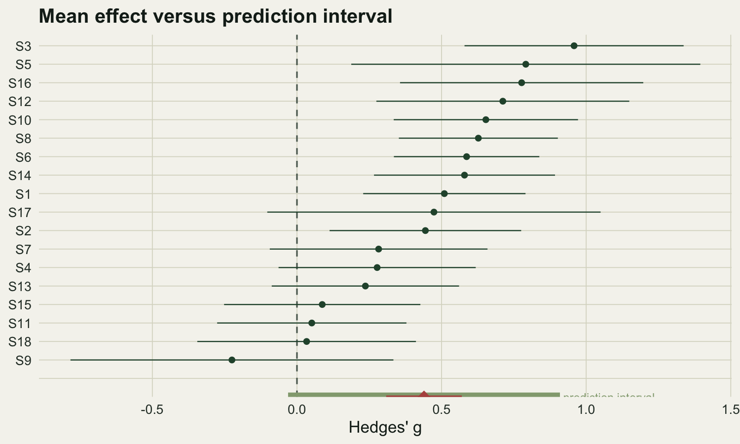
The confidence interval for the mean and the prediction interval answer different questions. The confidence interval asks where the average effect lies. The prediction interval asks where the true effect of a new, exchangeable study would fall, so it adds the between-study variance to the uncertainty in the mean and uses a t-distribution on k minus two degrees of freedom (IntHout et al. 2016).

ws  <- 1 / (v + tau2)
mre <- sum(ws * g) / sum(ws); se_re <- sqrt(1 / sum(ws))
ci  <- mre + c(-1, 1) * 1.96 * se_re                       # interval for the mean
pri <- mre + c(-1, 1) * qt(.975, k - 2) * sqrt(tau2 + se_re^2)  # prediction interval
rbind(mean_CI = ci, prediction = pri)

                 [,1]      [,2]
mean_CI     0.3084924 0.5700751
prediction -0.0307303 0.9092978

The mean sits at 0.439 with a confidence interval from 0.308 to 0.57, width 0.262. The prediction interval is far wider, from -0.031 to 0.909, a width of 0.94, about 3.6 times the confidence interval. That width is the honest statement of how much a new study might differ, and it is set by tau, not by I-squared.

se <- sqrt(v); ord <- order(g)
fdat <- data.frame(
  lab = factor(paste0("S", seq_len(k))[ord], levels = paste0("S", seq_len(k))[ord]),
  est = g[ord], lo = g[ord] - 1.96 * se[ord], hi = g[ord] + 1.96 * se[ord])
ggplot(fdat, aes(est, lab)) +
  geom_vline(xintercept = 0, linetype = "dashed", colour = pal$faint) +
  annotate("segment", x = pri[1], xend = pri[2], y = 0, yend = 0,
           colour = pal$sage, linewidth = 3) +
  geom_pointrange(aes(xmin = lo, xmax = hi), colour = pal$forest,
                  linewidth = 0.4, fatten = 1.6) +
  annotate("point", x = mre, y = 0, shape = 18, size = 4, colour = pal$warn) +
  annotate("segment", x = ci[1], xend = ci[2], y = 0, yend = 0,
           colour = pal$warn, linewidth = 1) +
  annotate("text", x = pri[2], y = 0, label = " prediction interval",
           hjust = 0, size = 3, colour = pal$sage) +
  scale_y_discrete(limits = c("", levels(fdat$lab))) +
  labs(x = "Hedges' g", y = NULL, title = "Mean effect versus prediction interval") +
  theme_te()

Figure 1: Forest plot with the pooled mean (red diamond, narrow confidence interval) and the prediction interval (sage bar), which spans where a new study’s true effect would fall. The prediction interval is in the units of the effect and is much wider than the confidence interval for the mean.

Why I-squared can mislead

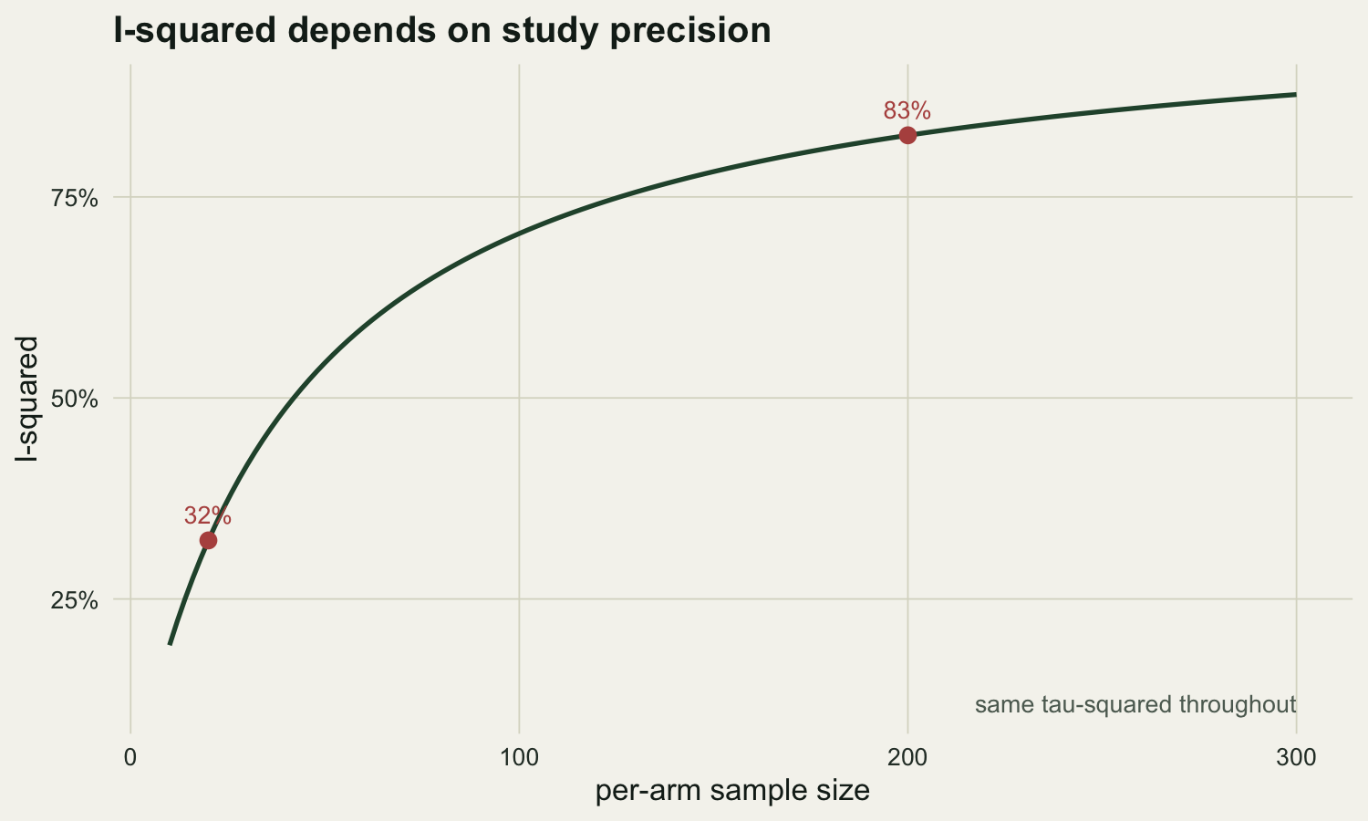
I-squared is the ratio of between-study variance to total variance, tau-squared over tau-squared plus a typical sampling variance. The sampling variance shrinks as studies grow, so the same absolute heterogeneity produces a larger I-squared when the studies are large. I-squared is therefore a relative measure and not a statement about the size of the effect-scale spread. The curve below fixes tau-squared at the true value and varies the per-arm sample size.

t2f  <- tau_true^2
nseq <- seq(10, 300, by = 2)
vtyp <- 2 / nseq + mu_true^2 / (4 * nseq)          # typical g variance at per-arm n
I2seq <- t2f / (t2f + vtyp)
mark  <- data.frame(nn = c(20, 200),
                    ii = t2f / (t2f + (2 / c(20, 200) + mu_true^2 / (4 * c(20, 200)))))
ggplot(data.frame(nn = nseq, ii = I2seq), aes(nn, ii)) +
  geom_line(colour = pal$forest, linewidth = 0.9) +
  geom_point(data = mark, aes(nn, ii), colour = pal$warn, size = 2.6) +
  geom_text(data = mark, aes(nn, ii, label = sprintf("%.0f%%", 100 * ii)),
            colour = pal$warn, vjust = -1, size = 3.4) +
  annotate("text", x = 300, y = 0.12, hjust = 1,
           label = "same tau-squared throughout", colour = pal$faint, size = 3.4) +
  labs(x = "per-arm sample size", y = "I-squared",
       title = "I-squared depends on study precision") +
  scale_y_continuous(labels = function(x) sprintf("%.0f%%", 100 * x)) +
  theme_te()

Figure 2: I-squared against per-arm sample size at a fixed between-study variance. The same tau-squared yields a low I-squared with small studies and a high one with large studies, so I-squared alone does not measure absolute heterogeneity.

At the same tau-squared, small studies of about 20 per arm give an I-squared near 32%, while large studies of about 200 per arm give an I-squared near 83%. The heterogeneity in effect-scale units has not changed. This is why an I-squared of ninety per cent from a set of large trials can be less consequential than one of fifty per cent from a set of small ones, and why the prediction interval, expressed in the units of the effect, is the safer summary to report and to interpret.

Honest limits

The test-based interval for I-squared and the Q-profile interval for tau-squared both assume the within-study variances are known, which is an approximation that weakens with very small studies. Q itself has low power to detect heterogeneity when k is small, so a non-significant Q is not evidence that the studies agree. None of these quantities tells you the cause of the disagreement; that is the job of meta-regression, which the next tutorial takes up.

Where to go next

If the studies vary, a study-level covariate may explain part of the variation. Meta-regression fits an effect on a moderator while keeping the residual between-study variance, and reports how much of the heterogeneity the moderator absorbs. After that, a funnel-plot check asks whether the studies in hand are a fair sample of the evidence, or whether small studies with inconvenient results are missing.

Related tutorials

• Random-effects meta-analysis in R
• Meta-regression with moderators
• Checking for publication bias
• When not to use the Shannon index

References

• Cochran WG 1954. Biometrics 10(1):101-129 (10.2307/3001666)
• Higgins JPT, Thompson SG 2002. Statistics in Medicine 21(11):1539-1558 (10.1002/sim.1186)
• Higgins JPT, Thompson SG, Deeks JJ, Altman DG 2003. BMJ 327(7414):557-560 (10.1136/bmj.327.7414.557)
• Viechtbauer W 2007. Statistics in Medicine 26(1):37-52 (10.1002/sim.2514)
• IntHout J, Ioannidis JPA, Rovers MM, Goeman JJ 2016. BMJ Open 6(7):e010247 (10.1136/bmjopen-2015-010247)
• Borenstein M, Hedges LV, Higgins JPT, Rothstein HR 2009. Introduction to Meta-Analysis. ISBN 978-0-470-05724-7