Checking for publication bias

Detect small-study effects in an ecological meta-analysis with base R: funnel plots, Egger’s regression test, and trim-and-fill, with the limits of each.

Every quantity in a meta-analysis, the pooled effect, the heterogeneity, the moderator slopes, assumes the studies in hand are a fair sample of the work that was done. They often are not. Small studies with null or wrong-signed results are less likely to be written up and published, so the literature over-represents large positive effects and the pooled estimate is pulled away from the truth. This post closes the meta-analysis thread with the standard checks for that problem in base R: the funnel plot, Egger’s regression test, and trim-and-fill. It also shows where these checks stop, because funnel asymmetry has several causes and none of them is proven by the plot alone.

Two literatures: one fair, one filtered

We build two sets of studies with the same true effect of 0.3. The first keeps every study. The second mimics selective publication: a study is published for certain if its effect is significantly positive, and only with low probability otherwise, which quietly removes small studies with unremarkable results.

sim_study <- function(theta, ni) {
  x1 <- rnorm(ni, 0, 1); x2 <- rnorm(ni, theta, 1)
  sp <- sqrt(((ni - 1) * sd(x1)^2 + (ni - 1) * sd(x2)^2) / (2 * ni - 2))
  d  <- (mean(x2) - mean(x1)) / sp
  J  <- 1 - 3 / (4 * (2 * ni - 2) - 1)
  g  <- J * d
  vd <- (2 * ni) / (ni * ni) + d^2 / (2 * (2 * ni))
  c(g = g, v = J^2 * vd)
}
wmean <- function(y, v) sum(y / v) / sum(1 / v)
mu <- 0.30

## unbiased: keep all 30 studies
set.seed(50)
ku <- 30; nu <- sample(10:90, ku, replace = TRUE)
gv <- t(mapply(sim_study, rnorm(ku, mu, 0.05), nu))
gu <- gv[, "g"]; seu <- sqrt(gv[, "v"])

## biased: simulate a pool, publish significant-positive for sure, else with p = 0.08
set.seed(302)
pool <- 260; np <- sample(10:90, pool, replace = TRUE)
gv <- t(mapply(sim_study, rnorm(pool, mu, 0.05), np))
gp <- gv[, "g"]; sep <- sqrt(gv[, "v"])
published <- (gp / sep > 1.64) | (runif(pool) < 0.08)
idx <- which(published)[1:32]
gb <- gp[idx]; seb <- sep[idx]
c(pooled_unbiased = wmean(gu, seu^2), pooled_biased = wmean(gb, seb^2))

pooled_unbiased   pooled_biased 
      0.3024662       0.4299897 

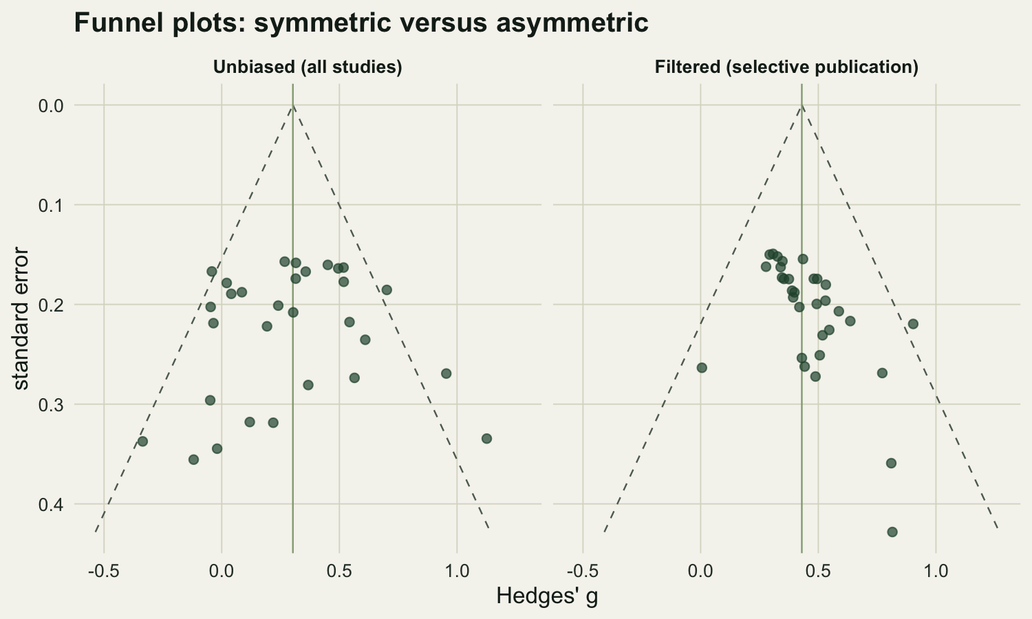
The unbiased set pools to 0.302, close to the true 0.3. The filtered set pools to 0.43, well above the truth: selective publication alone has inflated the apparent effect by about half. A funnel plot makes the mechanism visible.

fdat <- rbind(
  data.frame(g = gu, se = seu, set = "Unbiased (all studies)"),
  data.frame(g = gb, se = seb, set = "Filtered (selective publication)"))
fdat$set <- factor(fdat$set, levels = c("Unbiased (all studies)",
                                         "Filtered (selective publication)"))
poolv <- c("Unbiased (all studies)" = wmean(gu, seu^2),
           "Filtered (selective publication)" = wmean(gb, seb^2))
sey  <- seq(0, max(fdat$se), length.out = 40)
edge <- do.call(rbind, lapply(names(poolv), function(nm) rbind(
  data.frame(x = poolv[nm] - 1.96 * sey, se = sey, set = nm, side = "l"),
  data.frame(x = poolv[nm] + 1.96 * sey, se = sey, set = nm, side = "r"))))
edge$set <- factor(edge$set, levels = levels(fdat$set))
cen <- data.frame(x = as.numeric(poolv), set = factor(names(poolv), levels = levels(fdat$set)))
ggplot(fdat, aes(g, se)) +
  geom_line(data = edge, aes(x, se, group = side), linetype = "dashed",
            colour = pal$faint, linewidth = 0.4) +
  geom_vline(data = cen, aes(xintercept = x), colour = pal$sage, linewidth = 0.4) +
  geom_point(colour = pal$forest, alpha = 0.7, size = 1.9) +
  scale_y_reverse() +
  facet_wrap(~ set) +
  labs(x = "Hedges' g", y = "standard error",
       title = "Funnel plots: symmetric versus asymmetric") +
  theme_te()

Figure 1: Funnel plots for the two sets of studies. Effect size on the x axis, standard error on the y axis (precise studies at the top). The dashed lines are the 95% pseudo-confidence funnel around the pooled effect. The unbiased set is symmetric; the filtered set has a gap at the bottom left where small, null or negative studies are missing.

Egger’s regression test

Egger’s test formalises the asymmetry. Regress each study’s standardised effect, g over its standard error, on its precision, one over the standard error. If the small studies are systematically off, the intercept departs from zero (Egger et al. 1997).

egger <- function(g, se) {
  m <- lm(I(g / se) ~ I(1 / se))
  s <- summary(m)$coefficients
  c(intercept = s[1, 1], se = s[1, 2], t = s[1, 3], p = s[1, 4])
}
eu <- egger(gu, seu)
eb <- egger(gb, seb)
rbind(unbiased = eu, biased = eb)

          intercept        se          t           p
unbiased -0.4201889 0.9884802 -0.4250858 0.674023271
biased    1.8322720 0.5334083  3.4350273 0.001753982

For the unbiased set the intercept is -0.42 (p = 0.67), consistent with no asymmetry. For the filtered set the intercept is 1.83 with p = 0.0018, so the test flags the asymmetry the funnel showed.

Trim-and-fill

Trim-and-fill estimates how many studies are missing, imputes their mirror images, and re-estimates the pooled effect (Duval and Tweedie 2000). The L0 estimator below trims the most extreme studies on the heavy side, recomputes the centre, and repeats until the count of missing studies settles, then fills in the reflected points.

trimfill <- function(g, se) {
  v <- se^2; k <- length(g); mu0 <- wmean(g, v)
  side <- if (sum(sign(g - mu0)) >= 0) 1 else -1     # 1 = excess on the right
  yy <- side * g; ord <- order(yy)
  k0 <- 0; k0o <- -1; mu <- mu0; it <- 0
  while (k0 != k0o && it < 100) {
    it <- it + 1; k0o <- k0
    keep <- if (k0 > 0) ord[1:(k - k0)] else ord
    mu  <- wmean(g[keep], v[keep]); cen <- side * mu
    dd  <- yy - cen; r <- rank(abs(dd)); Tn <- sum(r[dd > 0])
    k0  <- max(0, round((4 * Tn - k * (k + 1)) / (2 * k - 1)))
  }
  cen <- side * mu
  if (k0 > 0) {
    ex <- ord[(k - k0 + 1):k]
    ga <- c(g, side * (2 * cen - yy[ex])); sa <- c(se, se[ex])
    imp <- (k + 1):(k + k0)
  } else { ga <- g; sa <- se; imp <- integer(0) }
  list(k0 = k0, mu_naive = wmean(g, v), mu_fill = wmean(ga, sa^2),
       ga = ga, sa = sa, imp = imp)
}
tu <- trimfill(gu, seu)
tb <- trimfill(gb, seb)
rbind(unbiased = c(k0 = tu$k0, naive = tu$mu_naive, filled = tu$mu_fill),
      biased   = c(k0 = tb$k0, naive = tb$mu_naive, filled = tb$mu_fill))

         k0     naive    filled
unbiased  0 0.3024662 0.3024662
biased   10 0.4299897 0.3736799

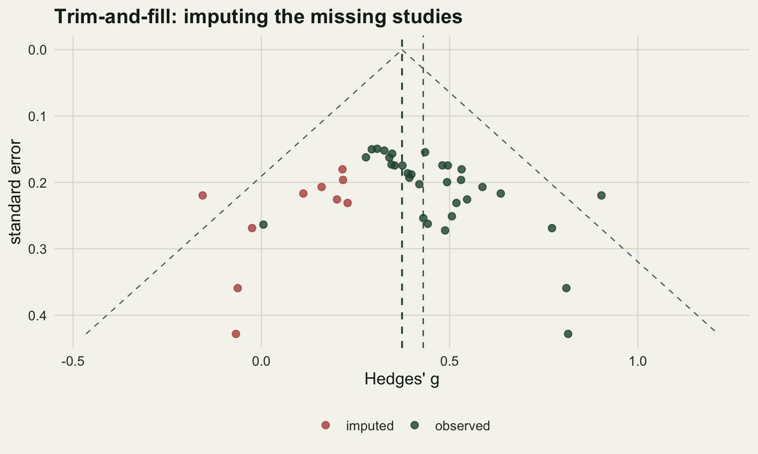
The unbiased set needs no filling: trim-and-fill imputes 0 studies and leaves the estimate at 0.302. The filtered set imputes 10 missing studies and pulls the pooled effect down from 0.43 to 0.374, back toward the true 0.3 though not all the way. The figure shows the imputed studies filling the empty corner of the funnel.

tf <- data.frame(g = tb$ga, se = tb$sa,
                 kind = ifelse(seq_along(tb$ga) %in% tb$imp, "imputed", "observed"))
sey2 <- seq(0, max(tf$se), length.out = 40)
edge2 <- rbind(
  data.frame(x = tb$mu_fill - 1.96 * sey2, se = sey2, side = "l"),
  data.frame(x = tb$mu_fill + 1.96 * sey2, se = sey2, side = "r"))
ggplot(tf, aes(g, se, colour = kind)) +
  geom_line(data = edge2, aes(x, se, group = side), inherit.aes = FALSE,
            linetype = "dashed", colour = pal$faint, linewidth = 0.4) +
  geom_vline(xintercept = tb$mu_naive, colour = pal$faint,
             linetype = "dashed", linewidth = 0.5) +
  geom_vline(xintercept = tb$mu_fill, colour = pal$forest,
             linetype = "dashed", linewidth = 0.6) +
  geom_point(size = 2.1, alpha = 0.8) +
  scale_y_reverse() +
  scale_colour_manual(values = c(observed = pal$forest, imputed = pal$warn),
                      name = NULL) +
  labs(x = "Hedges' g", y = "standard error",
       title = "Trim-and-fill: imputing the missing studies") +
  theme_te()

Figure 2: Trim-and-fill on the filtered set. Observed studies in green, imputed mirror studies in red, with the naive pooled estimate (grey) and the adjusted estimate after filling (green). The imputed points occupy the gap and shift the summary toward the null.

Honest limits

These are checks, not proofs, and they are easy to over-read. Funnel asymmetry has several causes besides publication bias: real heterogeneity, where small studies genuinely differ from large ones, produces the same pattern, and so can a link between study size and quality, or plain chance when the number of studies is small. Egger’s test has low power with few studies and can misfire when the effect metric is tied to its own standard error, as happens with log odds ratios and standardised mean differences. Trim-and-fill is a sensitivity analysis, not a correction to be trusted: it assumes the asymmetry is due to missing studies, it can add studies that never existed when the true cause is heterogeneity, and its adjusted estimate here still sits above the truth. Read together, these tools answer a narrow question well, whether the effect depends on study size, and leave the harder question, why, to judgement and to the design of the review itself.

The meta-analysis thread, end to end

Across four tutorials the pieces fit together. A random-effects model pools effect sizes and carries the between-study variance so its interval is honest. The heterogeneity tools describe that variance in the units of the effect, where a prediction interval says more than I-squared. Meta-regression asks whether a moderator explains the spread, and controls the false positives that a fixed-effect fit would invent. And the publication-bias checks ask whether the studies were a fair sample to begin with. Each step guards the step before it, which is the whole point of a careful synthesis.

Related tutorials

• Random-effects meta-analysis in R
• Heterogeneity in meta-analysis
• Meta-regression with moderators
• Bootstrap confidence intervals

References

• Egger M, Davey Smith G, Schneider M, Minder C 1997. BMJ 315(7109):629-634 (10.1136/bmj.315.7109.629)
• Duval S, Tweedie R 2000. Biometrics 56(2):455-463 (10.1111/j.0006-341X.2000.00455.x)
• Sterne JAC, Sutton AJ, Ioannidis JPA, et al. 2011. BMJ 343:d4002 (10.1136/bmj.d4002)
• Nakagawa S, Santos ESA 2012. Evolutionary Ecology 26(5):1253-1274 (10.1007/s10682-012-9555-5)
• Koricheva J, Gurevitch J, Mengersen K 2013. Handbook of Meta-analysis in Ecology and Evolution. ISBN 978-0-691-13729-4
• Borenstein M, Hedges LV, Higgins JPT, Rothstein HR 2009. Introduction to Meta-Analysis. ISBN 978-0-470-05724-7