Meta-regression with moderators

Explain heterogeneity with a study-level moderator in base R: weighted meta-regression, residual tau-squared, an R-squared analogue, and error control.

A random-effects model measures how much studies disagree, but not why. Meta-regression asks whether a study-level covariate, a moderator, accounts for some of the spread: latitude, study duration, mean body size, sampling method. It is a weighted regression of the effect sizes on the moderator, with the between-study variance kept as a residual term. This post builds it in base R, reports how much heterogeneity the moderator absorbs, and shows the common mistake of running a meta-regression without that residual term, which turns real heterogeneity into false moderator effects.

A moderator that drives the effect

We simulate 25 studies whose true effect depends on a standardised moderator x, with intercept 0.1 and slope 0.35, plus residual between-study noise with standard deviation 0.15. Each study reports a Hedges’ g and its known sampling variance.

sim_study <- function(theta, ni) {
  x1 <- rnorm(ni, 0, 1); x2 <- rnorm(ni, theta, 1)
  sp <- sqrt(((ni - 1) * sd(x1)^2 + (ni - 1) * sd(x2)^2) / (2 * ni - 2))
  d  <- (mean(x2) - mean(x1)) / sp
  J  <- 1 - 3 / (4 * (2 * ni - 2) - 1)
  g  <- J * d
  vd <- (2 * ni) / (ni * ni) + d^2 / (2 * (2 * ni))
  c(g = g, v = J^2 * vd)
}
set.seed(153)
k <- 25; b0 <- 0.10; b1 <- 0.35; tau_r <- 0.15
x <- scale(runif(k, -2, 2))[, 1]              # standardised moderator
n <- sample(15:120, k, replace = TRUE)
theta_i <- b0 + b1 * x + rnorm(k, 0, tau_r)   # true effect depends on x
gv <- t(mapply(sim_study, theta_i, n))
g  <- gv[, "g"]; v <- gv[, "v"]

Fitting the meta-regression

Given a residual between-study variance tau-squared, the coefficients are a generalised least-squares fit with weights equal to one over v plus tau-squared. We estimate tau-squared by REML, maximising the restricted log-likelihood over a one-parameter search, then read the coefficients and their standard errors from the weighted normal equations.

mreg <- function(y, v, X) {
  reml <- function(t2) {
    W   <- 1 / (v + t2); XtW <- t(X * W)
    b   <- solve(XtW %*% X, XtW %*% y); r <- y - X %*% b
    -0.5 * sum(log(v + t2)) - 0.5 * log(det(XtW %*% X)) - 0.5 * sum(W * r^2)
  }
  t2  <- optimize(reml, c(0, 10), maximum = TRUE)$maximum
  W   <- 1 / (v + t2); XtW <- t(X * W)
  Vb  <- solve(XtW %*% X); b <- Vb %*% (XtW %*% y)
  list(b = as.vector(b), se = sqrt(diag(Vb)), tau2 = t2, Vb = Vb)
}
X   <- cbind(1, x)
fit <- mreg(g, v, X)
QM  <- (fit$b[2] / fit$se[2])^2                 # Wald test for the slope
pQM <- pchisq(QM, 1, lower.tail = FALSE)
c(intercept = fit$b[1], slope = fit$b[2], se_slope = fit$se[2], QM = QM, p = pQM)

   intercept        slope   se_slope.x         QM.x          p.x 
1.831307e-01 3.499952e-01 5.612252e-02 3.889106e+01 4.481271e-10 

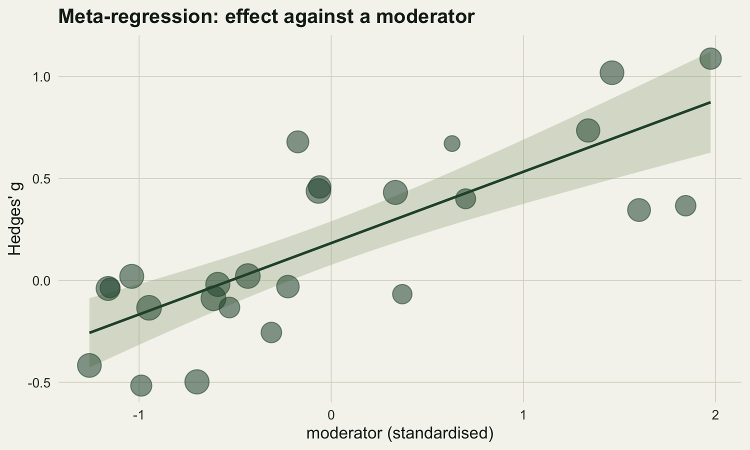
The estimated slope is 0.35 with a standard error of 0.056, recovering the true 0.35. The Wald test gives QM equal to 38.9 on one degree of freedom (p = 4.5^{-10}), so the moderator is clearly related to the effect.

How much heterogeneity does it explain?

Fit an intercept-only random-effects model to get the total between-study variance, then compare it with the residual left after the moderator. The proportion removed is an R-squared analogue for meta-analysis.

wf       <- 1 / v; mu_fe <- sum(wf * g) / sum(wf)
Q        <- sum(wf * (g - mu_fe)^2); Cc <- sum(wf) - sum(wf^2) / sum(wf)
tau2_tot <- max(0, (Q - (k - 1)) / Cc)          # total heterogeneity
tau2_res <- fit$tau2                            # residual after moderator
R2       <- max(0, (tau2_tot - tau2_res) / tau2_tot)
c(tau2_total = tau2_tot, tau2_residual = tau2_res, R2_analog = R2)

   tau2_total tau2_residual     R2_analog 
   0.15954880    0.04401851    0.72410630 

Total between-study variance is 0.16; after fitting the moderator the residual falls to 0.044, so the moderator accounts for about 72% of the heterogeneity. The rest is genuine residual variation among studies that share the same moderator value.

xg  <- seq(min(x), max(x), length.out = 100)
Xg  <- cbind(1, xg)
fitv <- as.vector(Xg %*% fit$b)
sef  <- sqrt(rowSums((Xg %*% fit$Vb) * Xg))
band <- data.frame(x = xg, y = fitv, lo = fitv - 1.96 * sef, hi = fitv + 1.96 * sef)
bub  <- data.frame(x = x, g = g, prec = 1 / (v + tau2_res))
ggplot(bub, aes(x, g)) +
  geom_ribbon(data = band, aes(x, ymin = lo, ymax = hi), inherit.aes = FALSE,
              fill = pal$sage, alpha = 0.30) +
  geom_line(data = band, aes(x, y), inherit.aes = FALSE,
            colour = pal$forest, linewidth = 0.9) +
  geom_point(aes(size = prec), colour = pal$forest, alpha = 0.55) +
  scale_size_area(max_size = 8, guide = "none") +
  labs(x = "moderator (standardised)", y = "Hedges' g",
       title = "Meta-regression: effect against a moderator") +
  theme_te()

Figure 1: Bubble plot of study effect against the moderator, with point area proportional to study precision and the fitted meta-regression line with its 95% band. Larger, more precise studies pull the line more strongly.

The mistake: ignoring the residual variance

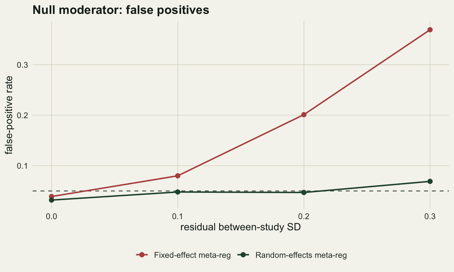
A tempting shortcut is to weight the regression only by within-study precision, one over v, and leave out the residual between-study variance. That is a fixed-effect meta-regression. When there is real residual heterogeneity, its standard errors are too small and the moderator test rejects far too often. We check this with a null moderator, one that has no true effect, and count how often each method declares it significant as the residual variance grows.

freg <- function(y, v, X) {                     # fixed-effect meta-regression
  W <- 1 / v; XtW <- t(X * W); Vb <- solve(XtW %*% X); b <- Vb %*% (XtW %*% y)
  list(b = as.vector(b), se = sqrt(diag(Vb)))
}
type_one <- function(tt, nsim = 1000) {
  fx <- 0; rx <- 0
  for (s in seq_len(nsim)) {
    xx <- scale(runif(k, -2, 2))[, 1]; nn <- sample(15:120, k, replace = TRUE)
    thh <- b0 + 0 * xx + rnorm(k, 0, tt)        # NULL slope
    gg <- numeric(k); vv <- numeric(k)
    for (i in seq_len(k)) { r <- sim_study(thh[i], nn[i]); gg[i] <- r[1]; vv[i] <- r[2] }
    XX <- cbind(1, xx)
    ff <- freg(gg, vv, XX); if (abs(ff$b[2] / ff$se[2]) > 1.96) fx <- fx + 1
    rr <- tryCatch(mreg(gg, vv, XX), error = function(e) NULL)
    if (!is.null(rr) && abs(rr$b[2] / rr$se[2]) > 1.96) rx <- rx + 1
  }
  c(fixed = fx / nsim, random = rx / nsim)
}
set.seed(4242)
grid <- c(0, 0.1, 0.2, 0.3)
t1tab <- as.data.frame(t(sapply(grid, type_one)))
t1tab$tau <- grid
round(t1tab[, c("tau", "fixed", "random")], 3)

  tau fixed random
1 0.0 0.039  0.032
2 0.1 0.080  0.048
3 0.2 0.201  0.047
4 0.3 0.369  0.069

With no residual heterogeneity both methods reject the null moderator about five per cent of the time, as they should. As residual variation grows, the fixed-effect meta-regression climbs to a rejection rate of 36.9%, so a moderator with no real effect looks significant in more than a third of analyses. The random-effects meta-regression stays near five per cent throughout (6.9% at the largest residual variance). Leaving the residual term out does not make the analysis sharper; it manufactures moderator effects out of ordinary heterogeneity.

tdat <- rbind(
  data.frame(tau = grid, rate = t1tab$fixed, model = "Fixed-effect meta-reg"),
  data.frame(tau = grid, rate = t1tab$random, model = "Random-effects meta-reg"))
ggplot(tdat, aes(tau, rate, colour = model)) +
  geom_hline(yintercept = 0.05, linetype = "dashed", colour = pal$faint) +
  geom_line(linewidth = 0.8) + geom_point(size = 2.2) +
  scale_colour_manual(values = c("Fixed-effect meta-reg" = pal$warn,
                                 "Random-effects meta-reg" = pal$forest), name = NULL) +
  labs(x = "residual between-study SD", y = "false-positive rate",
       title = "Null moderator: false positives") +
  theme_te()

Figure 2: False-positive rate for a null moderator against residual between-study standard deviation. The fixed-effect meta-regression inflates badly as residual heterogeneity grows; the random-effects version holds near the nominal 0.05.

Honest limits

Even the random-effects meta-regression is slightly liberal at the largest residual variance with only 25 studies, the same small-sample effect seen with the pooled mean; the Knapp-Hartung adjustment, which uses a t-distribution and a rescaled variance, tightens the test and is the safer default. Two cautions matter more. Meta-regression with few studies over-fits easily, and a handful of moderators tested one after another will turn up a spurious winner; keep the number of moderators small relative to the number of studies. And an observed moderator is not a manipulated one: study-level covariates are often correlated with each other and with design features, so a significant moderator is an association, not a demonstrated cause.

Where to go next

Meta-regression assumes the studies in hand are a fair sample of the evidence. If small studies with null or inconvenient results never reached publication, every quantity so far, the pooled mean, the heterogeneity, and the moderator slopes, can be biased. The final tutorial in this thread builds the funnel plot, Egger’s test, and trim-and-fill to check for that.

Related tutorials

• Random-effects meta-analysis in R
• Heterogeneity in meta-analysis
• Checking for publication bias
• Model selection with AIC

References

• Thompson SG, Higgins JPT 2002. Statistics in Medicine 21(11):1559-1573 (10.1002/sim.1187)
• Knapp G, Hartung J 2003. Statistics in Medicine 22(17):2693-2710 (10.1002/sim.1482)
• Viechtbauer W 2005. Journal of Educational and Behavioral Statistics 30(3):261-293 (10.3102/10769986030003261)
• Nakagawa S, Santos ESA 2012. Evolutionary Ecology 26(5):1253-1274 (10.1007/s10682-012-9555-5)
• Borenstein M, Hedges LV, Higgins JPT, Rothstein HR 2009. Introduction to Meta-Analysis. ISBN 978-0-470-05724-7