---
title: "Random-effects meta-analysis in R"
description: "Pool effect sizes across ecological studies with a random-effects model in base R: Hedges' g, DerSimonian-Laird and REML tau-squared, forest plots and coverage."
date: "2026-05-24 09:00"
date-modified: "2026-09-27"
categories: [meta-analysis, ecology tutorial, R, effect size]
image: thumbnail.png
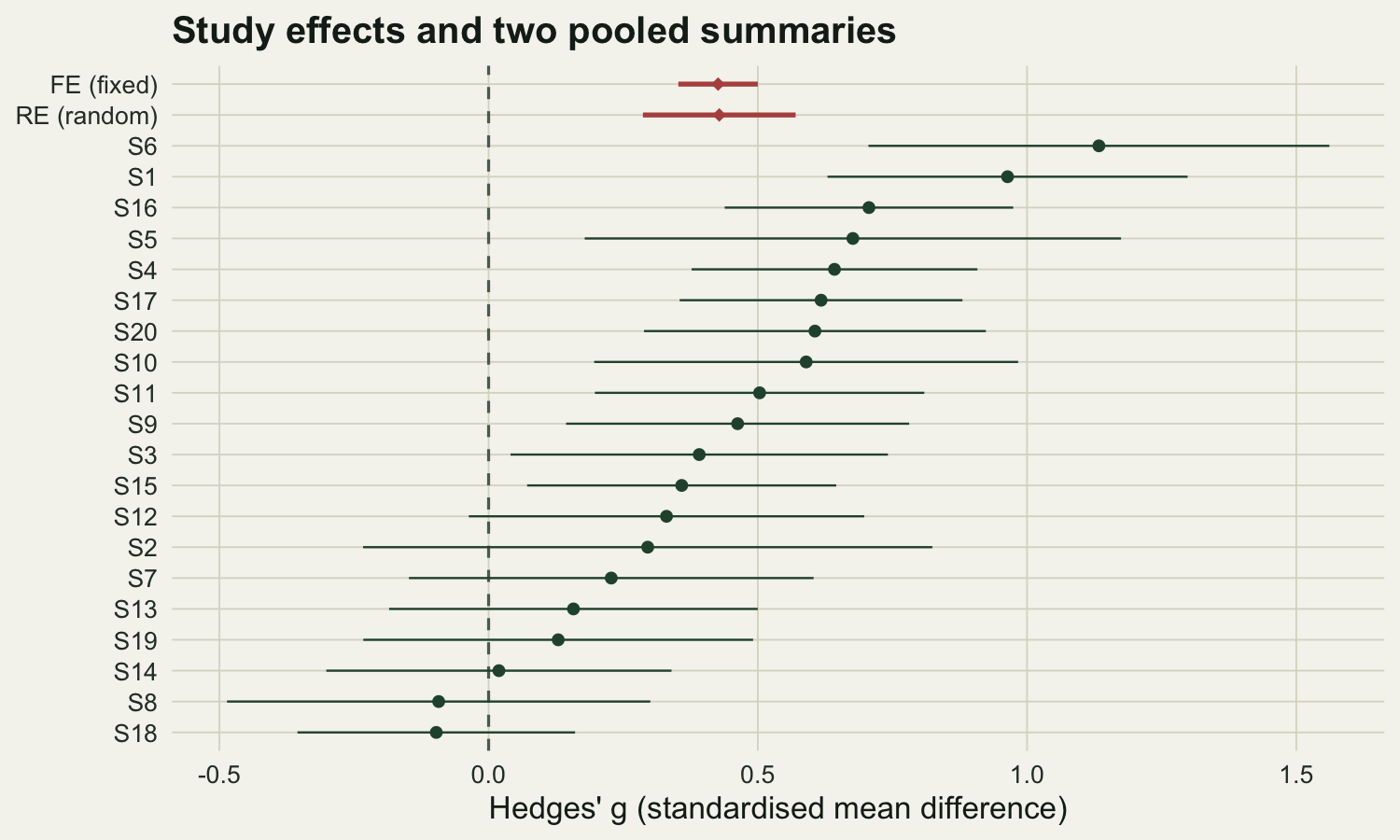
image-alt: "Forest plot of twenty study estimates above a single pooled summary row, the summary diamond near 0.4 on Hedges' g with its interval clear of the dashed zero line."
---
*Updated 27 September 2026: a new section, Four to six studies, measures the coverage of the default z interval against the Knapp-Hartung interval when a synthesis has only a handful of studies, and the Honest limits paragraph now points to it.*
A meta-analysis combines effect sizes from many studies into a single summary, with a measure of how much they disagree. In ecology the studies usually differ in site, species, and design, so the pooled estimate has to carry that spread rather than paper over it. This post builds a random-effects meta-analysis from scratch in base R and shows why the simpler fixed-effect model gives intervals that are too narrow once real between-study heterogeneity is present.
We use the standardised mean difference (Hedges' g) as the effect metric: the difference between a treatment group and a control group in pooled standard-deviation units, with a small-sample correction. Each study reports its own g and a within-study sampling variance v that we treat as known. The two models differ in one assumption. The fixed-effect (common-effect) model says every study estimates the same true effect and the only scatter is sampling noise. The random-effects model says each study has its own true effect drawn from a distribution with mean mu and variance tau-squared, so the summary target is the mean of that distribution.
```{r}
#| label: setup
#| code-fold: true
#| code-summary: "Setup: packages, colours and plot theme"
#| results: hide
#| message: false
#| warning: false
library(ggplot2)
knitr::opts_chunk$set(echo = TRUE, message = FALSE, warning = FALSE,
                      fig.width = 7.5, fig.height = 4.5, dpi = 100)
pal <- list(ink = "#16241d", body = "#2c3a31", forest = "#275139",
            label = "#46604a", sage = "#93a87f", paper = "#f5f4ee",
            line = "#dad9ca", faint = "#5d6b61", gold = "#cda23f",
            mown = "#2f8f63", warn = "#b5534e", low = "#c9b458", high = "#1d5b4e")
theme_te <- function(base_size = 12) {
  theme_minimal(base_size = base_size) +
    theme(panel.grid.minor = element_blank(),
          panel.grid.major = element_line(colour = pal$line, linewidth = 0.3),
          plot.background = element_rect(fill = pal$paper, colour = NA),
          panel.background = element_rect(fill = pal$paper, colour = NA),
          axis.text = element_text(colour = pal$body),
          axis.title = element_text(colour = pal$ink),
          plot.title = element_text(colour = pal$ink, face = "bold"),
          plot.subtitle = element_text(colour = pal$faint),
          legend.position = "bottom",
          legend.text = element_text(colour = pal$body),
          legend.title = element_text(colour = pal$ink))
}
```
```{r}
#| label: sci-tex-helper
#| include: false
sci_tex <- function(x, digits = 2) {
s <- formatC(x, format = "e", digits = digits)
paste0("$", sub("e.*", "", s), " \\times 10^{", as.integer(sub(".*e", "", s)), "}$")
}
```
## Simulating a set of studies
We simulate `r 20` studies. Each has a true effect drawn from a normal distribution with mean `r 0.40` and between-study standard deviation `r 0.25` (so tau-squared is `r 0.0625`). Sample sizes vary from study to study, which is what gives a meta-analysis its mix of precise and imprecise estimates. For each study we generate the raw group data, compute Cohen's d from the pooled standard deviation, apply the Hedges small-sample correction J, and record the large-sample variance of g.
```{r}
#| label: simulate
set.seed(151)
mu_true <- 0.40; tau_true <- 0.25; k <- 20
n <- sample(15:120, k, replace = TRUE)          # per-study sample size (per arm)

sim_study <- function(theta, ni) {
  x1 <- rnorm(ni, 0, 1)                          # control arm
  x2 <- rnorm(ni, theta, 1)                      # treatment arm
  sp <- sqrt(((ni - 1) * sd(x1)^2 + (ni - 1) * sd(x2)^2) / (2 * ni - 2))
  d  <- (mean(x2) - mean(x1)) / sp               # Cohen's d
  J  <- 1 - 3 / (4 * (2 * ni - 2) - 1)           # small-sample correction
  g  <- J * d                                    # Hedges' g
  vd <- (2 * ni) / (ni * ni) + d^2 / (2 * (2 * ni))
  c(g = g, v = J^2 * vd)                         # g and its sampling variance
}

theta_i <- rnorm(k, mu_true, tau_true)           # each study's own true effect
gv <- t(mapply(sim_study, theta_i, n))
g  <- gv[, "g"]; v <- gv[, "v"]
se <- sqrt(v)
round(cbind(n, g = g, se = se)[1:6, ], 3)
```
## Fixed-effect model
The fixed-effect estimate is a precision-weighted average, with weights equal to the inverse sampling variance. Precise studies (large n, small v) count more.
```{r}
#| label: fixed-effect
wf    <- 1 / v
mu_fe <- sum(wf * g) / sum(wf)
se_fe <- sqrt(1 / sum(wf))
ci_fe <- mu_fe + c(-1, 1) * 1.96 * se_fe
c(estimate = mu_fe, se = se_fe, lower = ci_fe[1], upper = ci_fe[2])
```
The fixed-effect summary is `r round(mu_fe, 3)` with a 95% interval from `r round(ci_fe[1], 3)` to `r round(ci_fe[2], 3)`, a width of `r round(diff(ci_fe), 3)`. That interval is only honest if the studies really do share one true effect. Cochran's Q tests that assumption: it is the weighted sum of squared deviations of each study from the fixed-effect summary, compared with a chi-squared distribution on k minus one degrees of freedom.
```{r}
#| label: q-test
Q   <- sum(wf * (g - mu_fe)^2)
dfQ <- k - 1
pQ  <- pchisq(Q, dfQ, lower.tail = FALSE)
c(Q = Q, df = dfQ, p = pQ)
```
Here Q is `r round(Q, 1)` on `r dfQ` degrees of freedom (p = `r sci_tex(pQ, 1)`), so the studies disagree by more than sampling noise alone. The fixed-effect interval ignores that disagreement and will be too narrow.
## Random-effects: DerSimonian-Laird
The random-effects model adds a between-study variance tau-squared to every study's weight, so the weights become one over v plus tau-squared. The classic moment estimator of DerSimonian and Laird (1986) reads tau-squared straight off the Q statistic.
```{r}
#| label: dersimonian-laird
Cc      <- sum(wf) - sum(wf^2) / sum(wf)
tau2_dl <- max(0, (Q - dfQ) / Cc)                # DerSimonian-Laird moment estimate
ws      <- 1 / (v + tau2_dl)                     # random-effects weights
mu_re   <- sum(ws * g) / sum(ws)
se_re   <- sqrt(1 / sum(ws))
ci_re   <- mu_re + c(-1, 1) * 1.96 * se_re
c(tau2 = tau2_dl, estimate = mu_re, se = se_re, lower = ci_re[1], upper = ci_re[2])
```
## Random-effects: REML
The moment estimator is quick but a maximum-likelihood approach is the modern default. Restricted maximum likelihood (REML) estimates tau-squared by maximising the restricted log-likelihood, which accounts for the estimation of mu (Viechtbauer 2005). It is a one-parameter search over tau-squared, easy to code with `optimize`.
```{r}
#| label: reml
reml_ll <- function(t2) {
  wi <- 1 / (v + t2)
  mh <- sum(wi * g) / sum(wi)
  -0.5 * sum(log(v + t2)) - 0.5 * log(sum(wi)) - 0.5 * sum(wi * (g - mh)^2)
}
opt       <- optimize(reml_ll, c(0, 5), maximum = TRUE)
tau2_reml <- opt$maximum
wr        <- 1 / (v + tau2_reml)
mu_reml   <- sum(wr * g) / sum(wr)
se_reml   <- sqrt(1 / sum(wr))
ci_reml   <- mu_reml + c(-1, 1) * 1.96 * se_reml
c(tau2 = tau2_reml, estimate = mu_reml, se = se_reml)
```
The two estimators of tau-squared agree closely here: `r round(tau2_dl, 3)` from DerSimonian-Laird and `r round(tau2_reml, 3)` from REML, both near the true `r 0.0625`. The random-effects summary is `r round(mu_re, 3)` with a 95% interval from `r round(ci_re[1], 3)` to `r round(ci_re[2], 3)`. That interval is `r round(diff(ci_re) / diff(ci_fe), 2)` times as wide as the fixed-effect one, because the between-study variance flows into the standard error. The point estimate barely moves; what changes is the honesty of the uncertainty.
```{r}
#| label: fig-re-forest
#| fig-cap: "Forest plot of 20 simulated studies (Hedges' g with 95% intervals), ordered by effect size, with the fixed-effect and random-effects pooled estimates. The random-effects interval is wider because it carries the between-study variance."
#| fig-alt: "Forest plot: twenty horizontal point-and-whisker rows for the studies, sorted by effect size, below two summary rows drawn at the top of the panel. The fixed-effect summary near 0.43 has a narrow interval; the random-effects summary at the same point has a visibly wider interval. A dashed vertical line marks zero effect."
ord <- order(g)
fdat <- data.frame(
  lab = factor(paste0("S", seq_len(k))[ord], levels = paste0("S", seq_len(k))[ord]),
  est = g[ord], lo = g[ord] - 1.96 * se[ord], hi = g[ord] + 1.96 * se[ord])
sdat <- data.frame(
  lab = factor(c("RE (random)", "FE (fixed)"),
               levels = c("RE (random)", "FE (fixed)")),
  est = c(mu_re, mu_fe), lo = c(ci_re[1], ci_fe[1]), hi = c(ci_re[2], ci_fe[2]))

ggplot(fdat, aes(est, lab)) +
  geom_vline(xintercept = 0, linetype = "dashed", colour = pal$faint) +
  geom_pointrange(aes(xmin = lo, xmax = hi), colour = pal$forest,
                  linewidth = 0.4, fatten = 1.6) +
  geom_pointrange(data = sdat, aes(xmin = lo, xmax = hi), colour = pal$warn,
                  shape = 18, linewidth = 0.9, fatten = 3.2) +
  labs(x = "Hedges' g (standardised mean difference)", y = NULL,
       title = "Study effects and two pooled summaries") +
  theme_te()
```
## Why the intervals differ: a coverage check
The claim that the fixed-effect interval is too narrow is testable. We repeat the whole exercise many times at several true values of tau, and record how often each model's 95% interval contains the true mu. A well-behaved interval should contain the truth about 95% of the time. For speed the coverage loop uses the DerSimonian-Laird estimator, which has a closed form.
```{r}
#| label: coverage
cover_at <- function(tt, nsim = 1200) {
  fe <- 0; re <- 0
  for (s in seq_len(nsim)) {
    th <- rnorm(k, mu_true, tt)
    gg <- numeric(k); vv <- numeric(k)
    for (i in seq_len(k)) { r <- sim_study(th[i], n[i]); gg[i] <- r[1]; vv[i] <- r[2] }
    wF <- 1 / vv; mF <- sum(wF * gg) / sum(wF); sF <- sqrt(1 / sum(wF))
    if (abs(mF - mu_true) <= 1.96 * sF) fe <- fe + 1
    QQ <- sum(wF * (gg - mF)^2); CC <- sum(wF) - sum(wF^2) / sum(wF)
    t2 <- max(0, (QQ - (k - 1)) / CC); wS <- 1 / (vv + t2)
    mR <- sum(wS * gg) / sum(wS); sR <- sqrt(1 / sum(wS))
    if (abs(mR - mu_true) <= 1.96 * sR) re <- re + 1
  }
  c(fe = fe / nsim, re = re / nsim)
}
set.seed(2718)
grid   <- c(0, 0.1, 0.2, 0.3, 0.4)
covtab <- as.data.frame(t(sapply(grid, cover_at)))
covtab$tau <- grid
round(covtab[, c("tau", "fe", "re")], 3)
```
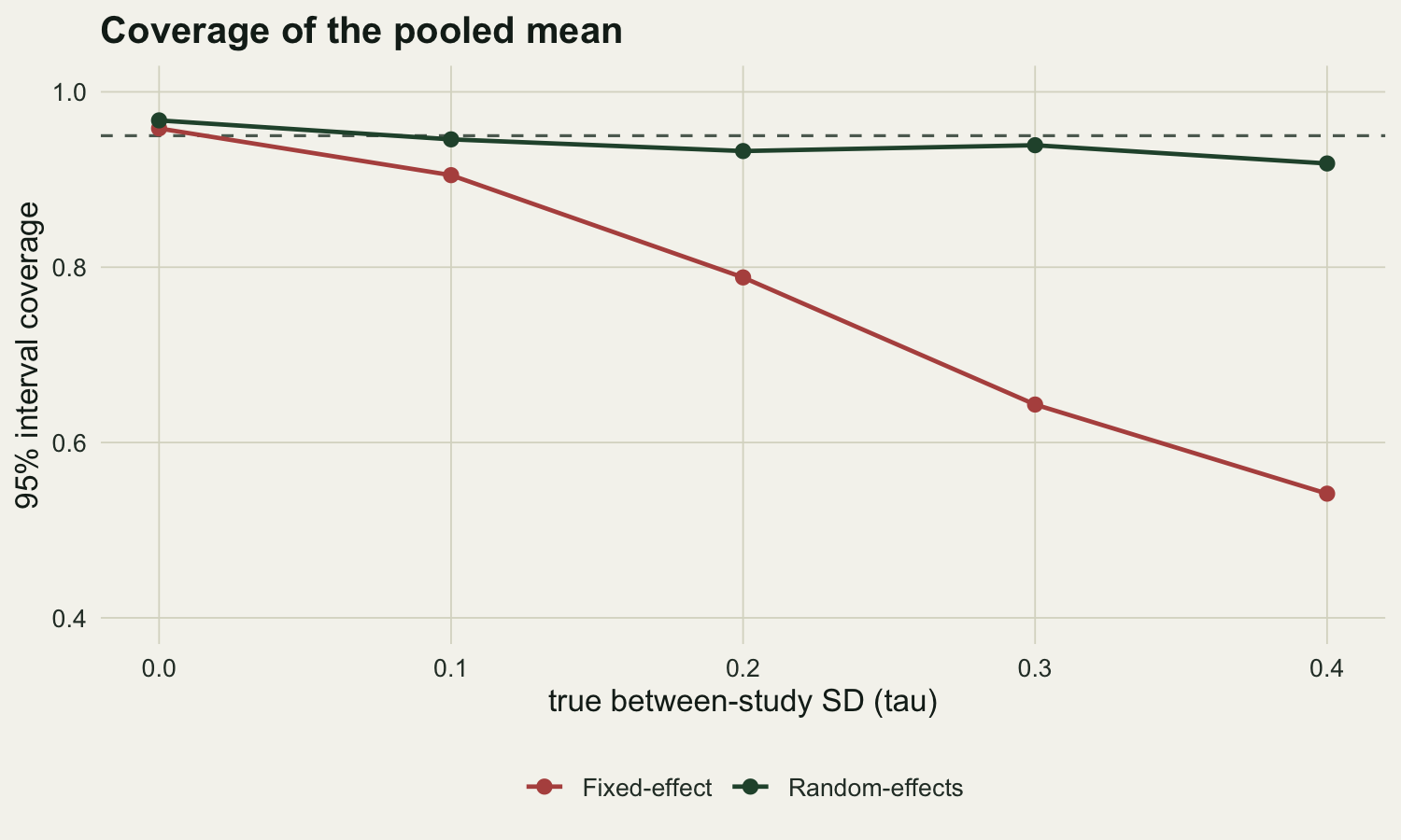
At tau equal to zero the two models agree and both sit near the nominal `r 0.95`. As between-study variance grows the fixed-effect interval decays: its coverage falls from `r sprintf("%.3f", covtab$fe[covtab$tau == 0])` to `r sprintf("%.3f", covtab$fe[covtab$tau == 0.4])`, so at the largest heterogeneity it misses the truth in nearly half of all meta-analyses. The random-effects interval holds much closer to nominal across the range (`r sprintf("%.3f", covtab$re[covtab$tau == 0.4])` at the largest tau). The lesson is direct: with heterogeneous studies, a fixed-effect interval understates uncertainty, and the size of that error grows with the heterogeneity.
```{r}
#| label: fig-re-coverage
#| fig-cap: "Interval coverage of the pooled mean against true between-study standard deviation, from simulation. Fixed-effect coverage collapses as heterogeneity grows; random-effects coverage stays near the nominal 0.95."
#| fig-alt: "Line chart with true between-study standard deviation on the x axis and interval coverage on the y axis. The fixed-effect line starts near 0.95 at zero and drops steeply to about 0.54. The random-effects line stays close to a dashed horizontal reference at 0.95 across the whole range."
cdat <- rbind(
  data.frame(tau = grid, cover = covtab$fe, model = "Fixed-effect"),
  data.frame(tau = grid, cover = covtab$re, model = "Random-effects"))
ggplot(cdat, aes(tau, cover, colour = model)) +
  geom_hline(yintercept = 0.95, linetype = "dashed", colour = pal$faint) +
  geom_line(linewidth = 0.8) + geom_point(size = 2.2) +
  scale_colour_manual(values = c("Fixed-effect" = pal$warn,
                                 "Random-effects" = pal$forest), name = NULL) +
  labs(x = "true between-study SD (tau)", y = "95% interval coverage",
       title = "Coverage of the pooled mean") +
  coord_cartesian(ylim = c(0.4, 1)) +
  theme_te()
```
## Four to six studies: the z interval against Knapp-Hartung
Twenty studies already left the z interval a little short at the largest tau above (`r sprintf("%.3f", covtab$re[covtab$tau == 0.4])`). A subgroup, a handful of field experiments or one taxon's slice of a review often leaves four to six. The chunk below reruns the coverage loop with the first four, six or ten of the twenty sample sizes above, at four of the same values of tau, and puts three intervals around the same DerSimonian-Laird estimate. The first is the z interval used so far. The second is the Knapp-Hartung interval (Knapp and Hartung 2003): it rescales the variance by q, the weighted squared deviations of the studies from the summary divided by k minus one, and uses a t quantile on k minus one degrees of freedom. The third is the "ad hoc" version that never lets q fall below one (Jackson and colleagues 2017). That the z interval undercovers with few studies and the t-based one comes much closer to nominal is a known result (IntHout and colleagues 2014); this is a demonstration of it on this post's generator. The loop also refits every synthesis with REML, which is what `rma()` in metafor uses by default, together with the z interval (metafor 4.4.0 and its 5.3-0 source on GitHub both have `method = "REML"` and `test = "z"`).
```{r}
#| label: few-studies
kh_at <- function(kk, tt, nsim = 2000) {
  tc <- qt(0.975, kk - 1)
  out <- matrix(NA, nsim, 8)
  for (s in seq_len(nsim)) {
    r  <- mapply(sim_study, rnorm(kk, mu_true, tt), n[seq_len(kk)])
    gg <- r[1, ]; vv <- r[2, ]
    wF <- 1 / vv; mF <- sum(wF * gg) / sum(wF)
    QQ <- sum(wF * (gg - mF)^2); CC <- sum(wF) - sum(wF^2) / sum(wF)
    t2 <- max(0, (QQ - (kk - 1)) / CC); wS <- 1 / (vv + t2)
    mR <- sum(wS * gg) / sum(wS); sR <- sqrt(1 / sum(wS))
    q  <- sum(wS * (gg - mR)^2) / (kk - 1)            # Knapp-Hartung scale
    rl <- function(x) { wi <- 1 / (vv + x); mh <- sum(wi * gg) / sum(wi)
      -0.5 * sum(log(vv + x)) - 0.5 * log(sum(wi)) - 0.5 * sum(wi * (gg - mh)^2) }
    wR <- 1 / (vv + optimize(rl, c(0, 5), maximum = TRUE)$maximum)
    mE <- sum(wR * gg) / sum(wR); qE <- sum(wR * (gg - mE)^2) / (kk - 1)
    out[s, ] <- c(abs(mR - mu_true) <= c(1.96, tc * sqrt(q), tc * sqrt(max(1, q))) * sR,
                  tc * sqrt(q) < 1.96, t2 == 0, q,
                  abs(mE - mu_true) <= c(1.96, tc * sqrt(qE)) * sqrt(1 / sum(wR)))
  }
  colnames(out) <- c("z", "kh", "adhoc", "narrow", "t2zero", "q", "z_reml", "kh_reml")
  stopifnot(out[, "narrow"] == (out[, "q"] < (1.96 / tc)^2),  # narrower iff q below the cut
            out[out[, "t2zero"] == 1, "q"] <= 1 + 1e-12)       # tau2 = 0 forces q <= 1
  out
}
set.seed(2719)
kh_grid <- expand.grid(tau = c(0, 0.1, 0.2, 0.4), kk = c(4, 6, 10))
kh_raw  <- lapply(seq_len(nrow(kh_grid)), function(i) kh_at(kh_grid$kk[i], kh_grid$tau[i]))
kh_tab  <- cbind(kh_grid, t(sapply(kh_raw, colMeans)))
kh_mcse <- sqrt(0.95 * 0.05 / 2000)                    # Monte Carlo SE near 0.95
kh_f3   <- function(x) sprintf("%.3f", round(x, 3))    # prose matches the table
kh_cut  <- (1.96 / qt(0.975, c(4, 6, 10) - 1))^2
kh_nz   <- unlist(lapply(kh_raw[kh_grid$tau <= 0.1], function(m) m[m[, "narrow"] == 1, "t2zero"]))
kh_nzc  <- c(narrow = length(kh_nz), tau2_positive = sum(kh_nz == 0))
kh_n4   <- colMeans(kh_raw[[1]][kh_raw[[1]][, "narrow"] == 1, c("z", "kh")])
kh_reml <- max(abs(kh_tab$z_reml - kh_tab$z), abs(kh_tab$kh_reml - kh_tab$kh))
kh_lo   <- kh_tab$kh[kh_tab$tau > 0 & kh_tab$kk <= 6]; stopifnot(all(kh_lo < 0.95))
round(kh_tab[, c("tau", "kk", "z", "kh", "adhoc", "narrow", "t2zero")], 3)
```
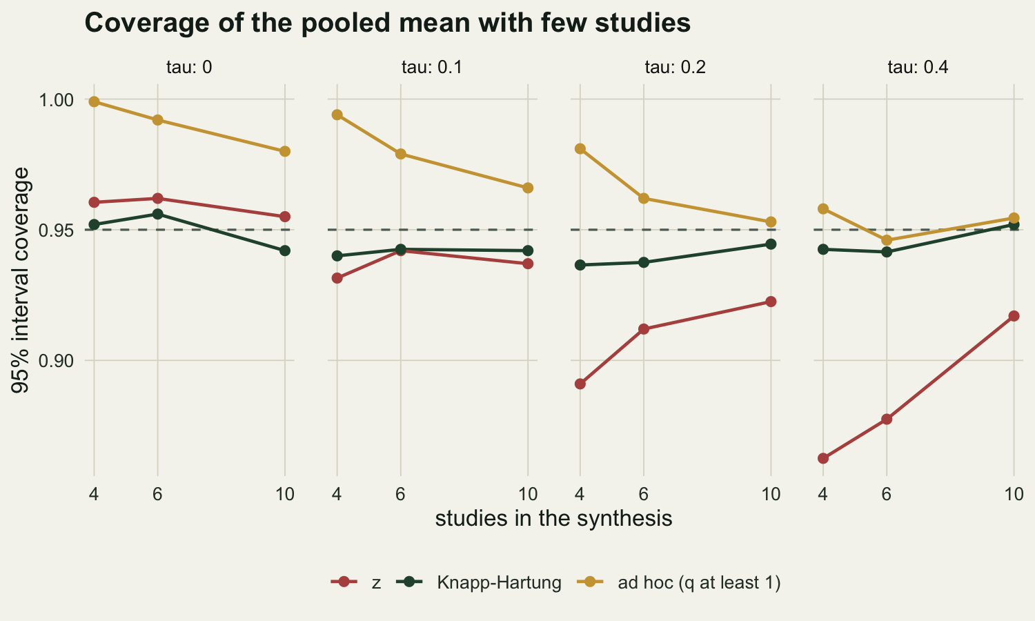
With a true between-study SD of 0.2 or 0.4 the z interval misses more often the fewer studies there are: at tau `r 0.4` it covers `r kh_f3(kh_tab$z[kh_tab$tau == 0.4 & kh_tab$kk == 4])`, `r kh_f3(kh_tab$z[kh_tab$tau == 0.4 & kh_tab$kk == 6])` and `r kh_f3(kh_tab$z[kh_tab$tau == 0.4 & kh_tab$kk == 10])` at four, six and ten studies, and at tau `r 0.2` it covers `r kh_f3(kh_tab$z[kh_tab$tau == 0.2 & kh_tab$kk == 4])` to `r kh_f3(kh_tab$z[kh_tab$tau == 0.2 & kh_tab$kk == 10])`. The Knapp-Hartung interval covers between `r kh_f3(min(kh_tab$kh))` and `r kh_f3(max(kh_tab$kh))` in every one of the twelve cells, against a Monte Carlo standard error of `r kh_f3(kh_mcse)` for a coverage near 0.95. With heterogeneity at four and six studies it sits a little below 0.95 in all six cells, `r kh_f3(mean(kh_lo))` on average against a Monte Carlo standard error of `r kh_f3(kh_mcse / sqrt(6))` for that average, so the repair is close, not exact. The ad hoc floor over-covers where the studies agree: `r kh_f3(kh_tab$adhoc[kh_tab$tau == 0 & kh_tab$kk == 4])` at four studies and no heterogeneity, `r kh_f3(kh_tab$adhoc[kh_tab$tau == 0 & kh_tab$kk == 10])` at ten. Refitting with REML moves neither the z nor the Knapp-Hartung coverage in any cell by more than `r kh_f3(kh_reml)`, so the picture is the same with metafor's default estimator.
```{r}
#| label: fig-re-few-studies
#| fig-cap: "Coverage of the pooled mean with four, six and ten studies at four values of the true between-study SD, from 2000 simulated syntheses per point, for the z interval, the Knapp-Hartung interval and its ad hoc version with q floored at one."
#| fig-alt: "Four line-chart panels side by side, headed tau: 0, tau: 0.1, tau: 0.2 and tau: 0.4, each plotting 95% interval coverage from about 0.86 to 1.00 against 4, 6 and 10 studies, with a dashed line at 0.95. A gold line for the ad hoc interval is highest in the first three panels, near 0.98 to 1.00 at four studies and falling towards the dashed line at ten; at tau 0.4 it runs near the dashed line. A dark green Knapp-Hartung line stays between about 0.94 and 0.96 in every panel. A red z line sits near 0.96 at tau 0 and near 0.93 to 0.94 at tau 0.1; at tau 0.2 and 0.4 it starts low at four studies, about 0.89 and 0.86, and rises to about 0.92 at ten."
kh_lab <- c("z", "Knapp-Hartung", "ad hoc (q at least 1)")
kdat <- data.frame(kh_tab[rep(1:12, 3), c("tau", "kk")], interval = rep(kh_lab, each = 12),
                   cover = c(kh_tab$z, kh_tab$kh, kh_tab$adhoc))
ggplot(kdat, aes(kk, cover, colour = interval)) +
  geom_hline(yintercept = 0.95, linetype = "dashed", colour = pal$faint) +
  geom_line(linewidth = 0.8) + geom_point(size = 2) +
  facet_wrap(~ tau, nrow = 1, labeller = label_both) +
  scale_x_continuous(breaks = c(4, 6, 10)) +
  scale_colour_manual(values = setNames(c(pal$warn, pal$forest, pal$gold), kh_lab),
                      breaks = kh_lab, name = NULL) +
  labs(x = "studies in the synthesis", y = "95% interval coverage",
       title = "Coverage of the pooled mean with few studies") +
  theme_te() + theme(panel.spacing = grid::unit(1.2, "lines"))
```
The Knapp-Hartung interval is not always the wider one. Its half-width is t times the square root of q times the standard error, against 1.96 times the standard error for z, so it is narrower exactly when q falls below (1.96 / t) squared: `r kh_f3(kh_cut[1])`, `r kh_f3(kh_cut[2])` and `r kh_f3(kh_cut[3])` at four, six and ten studies. How often q falls that low is not closed form. With no heterogeneity it happened in `r kh_f3(kh_tab$narrow[kh_tab$tau == 0 & kh_tab$kk == 4])`, `r kh_f3(kh_tab$narrow[kh_tab$tau == 0 & kh_tab$kk == 6])` and `r kh_f3(kh_tab$narrow[kh_tab$tau == 0 & kh_tab$kk == 10])` of syntheses at four, six and ten studies. It goes with an estimate of tau-squared of exactly zero: of the `r sprintf("%d", kh_nzc[["narrow"]])` narrower syntheses in the tau `r 0` and `r 0.1` cells, only `r sprintf("%d", kh_nzc[["tau2_positive"]])` had a positive estimate. The average coverage hides what happens in those syntheses: in the `r sprintf("%d", sum(kh_raw[[1]][, "narrow"]))` narrower syntheses at four studies and no heterogeneity the Knapp-Hartung interval covered `r kh_f3(kh_n4[["kh"]])` and the z interval `r kh_f3(kh_n4[["z"]])`. The ad hoc floor is there to stop exactly this (Jackson and colleagues 2017, their section 4.3). When the estimate of tau-squared is zero, q is Cochran's Q over k minus one and so at most one (the `stopifnot()` in the chunk checks this), the floor always applies, and the interval becomes the fixed-effect interval with a t multiplier, `r sprintf("%.2f", qt(0.975, 3) / 1.96)` times the z interval at four studies. That removes the narrow cases and produces the over-coverage above; it is a conservative choice, not a correct one. In metafor the three are one argument apart: `rma(yi, vi)` (REML and the z interval, the defaults), `rma(yi, vi, test = "knha")` and `rma(yi, vi, test = "adhoc")`.
All of these are intervals for the pooled mean, not for the effect at a new site, which is the job of the prediction interval in [prediction intervals for a new site](../prediction-interval-for-a-new-site/). The study variances here are treated as known; [little-replicated bioassays](../little-replicated-bioassays-in-a-meta-analysis/) scores the same Knapp-Hartung interval at five studies when each variance is itself estimated from three bottles, and [meta-regression with moderators](../meta-regression-moderators/) recommends the same adjustment for the moderator test.
## Honest limits
The random-effects interval here uses a normal (Wald) approximation with an estimated tau-squared. That approximation is good but not perfect: at the largest heterogeneity with only `r k` studies the coverage sits a little below nominal (`r sprintf("%.3f", covtab$re[covtab$tau == 0.4])`), the known slight anticonservatism of Wald intervals in small meta-analyses. The Knapp-Hartung adjustment, measured in the previous section, brings the average coverage to between `r kh_f3(min(kh_tab$kh))` and `r kh_f3(max(kh_tab$kh))` at four to ten studies, but it is not a uniformly wider interval, and its ad hoc floor removes the narrow cases at the price of over-coverage when the studies agree, most of all at four studies. Two further points matter more than the estimator. First, the effect metric is a modelling choice: Hedges' g, log response ratios, and correlation coefficients each have their own variance formula and their own interpretation, and they are not interchangeable. Second, the model assumes the studies are independent; multiple effects from one study or one research group break that assumption and call for a [multilevel meta-analysis](../dependent-effect-sizes-meta-analysis/).
## Where to go next
Heterogeneity is not a nuisance to be summarised in one number and forgotten. The next tutorial takes tau-squared apart with the Q statistic, I-squared, and the prediction interval, and shows why I-squared on its own can mislead. From there, meta-regression asks whether a study-level moderator explains some of the spread, and a funnel-plot check asks whether the set of studies is a fair sample of the evidence.
## References
- DerSimonian R, Laird N 1986. Controlled Clinical Trials 7(3):177-188 (10.1016/0197-2456(86)90046-2)
- Hedges LV 1981. Journal of Educational Statistics 6(2):107-128 (10.3102/10769986006002107)
- Viechtbauer W 2005. Journal of Educational and Behavioral Statistics 30(3):261-293 (10.3102/10769986030003261)
- Nakagawa S, Santos ESA 2012. Evolutionary Ecology 26(5):1253-1274 (10.1007/s10682-012-9555-5)
- Gurevitch J, Koricheva J, Nakagawa S, Stewart G 2018. Nature 555(7695):175-182 (10.1038/nature25753)
- Knapp G, Hartung J 2003. Statistics in Medicine 22(17):2693-2710 (10.1002/sim.1482)
- IntHout J, Ioannidis JPA, Borm GF 2014. BMC Medical Research Methodology 14:25 (10.1186/1471-2288-14-25)
- Jackson D, Law M, Rucker G, Schwarzer G 2017. Statistics in Medicine 36(25):3923-3934 (10.1002/sim.7411)
- Borenstein M, Hedges LV, Higgins JPT, Rothstein HR 2009. Introduction to Meta-Analysis. ISBN 978-0-470-05724-7
## Related tutorials
- [Heterogeneity in meta-analysis](../heterogeneity-in-meta-analysis/)
- [Meta-regression with moderators](../meta-regression-moderators/)
- [Dependent effect sizes in meta-analysis](../dependent-effect-sizes-meta-analysis/)
- [Prediction intervals for a new site in meta-analysis](../prediction-interval-for-a-new-site/)