library(ggplot2)
library(patchwork)

te_paper  <- "#f5f4ee"
te_ink    <- "#16241d"
te_body   <- "#2c3a31"
te_forest <- "#275139"
te_rust   <- "#b5534e"
te_gold   <- "#c9b458"
te_line   <- "#dad9ca"

theme_datasheet <- function() {
  theme_minimal(base_size = 12) +
    theme(plot.background  = element_rect(fill = te_paper, colour = NA),
          panel.background = element_rect(fill = te_paper, colour = NA),
          panel.grid.major = element_line(colour = te_line, linewidth = 0.3),
          panel.grid.minor = element_blank(),
          text             = element_text(colour = te_body),
          plot.title       = element_text(colour = te_ink, face = "bold"),
          plot.subtitle    = element_text(colour = te_body),
          axis.text        = element_text(colour = te_body))
}Selection models for publication bias
R
meta-analysis
publication bias
ecology tutorial
Fit the publication filter into the likelihood with base R, and measure how many ecological studies a weight-function selection model needs before it pays.
A synthesis of predator exclusion experiments ends up with twenty-three published effect sizes, standardised mean differences from plot counts ranging between ten and ninety. Pooling them by inverse variance gives an estimate, the funnel plot leans to the right, and Egger’s regression on the same studies flags the asymmetry at the conventional level with nothing to spare. At that point the review has a detection and no repair.
Trim-and-fill answers by imputing the studies it thinks are missing, which is a sensitivity analysis rather than an estimate. There is another route. If the filter that decides which studies get published is written into the likelihood, so that the density of a published effect is the ordinary density divided by the probability of surviving the filter, then the pooled effect is estimated under the filter instead of being doubted after the fact. The probability that a non-significant study still reaches print becomes a parameter with a value. That is an old idea (Iyengar and Greenhouse 1988; Hedges 1992) and it is not hard to code. The hard part is knowing when to use it, and the folklore answer, fit one once you have more than about ten studies, is a single slice through a surface. This post measures the surface, and it measures the bill the estimator hands you when there was no selection to correct.
The neighbouring posts on this site cover the two halves this one sits between. Checking for publication bias builds the funnel plot, Egger’s test and trim-and-fill, which detect. Parasite burdens truncated by host death builds the same likelihood machinery, a selection probability in the denominator fitted with optim, and reaches the opposite verdict about whether the selection parameter can be estimated at all. The contrast is the point, and it is settled below.
The published effects carry a step at the significance boundary
The generating process is the one the detection post used, written out as a model rather than as a demonstration. Each study has a true effect drawn around a grand mean, an observed effect drawn around that, and a standard error fixed by its sample size. A study is published for certain if its one-sided p value clears the threshold, and otherwise with probability w.
CRIT <- qnorm(0.975); alpha_1 <- pnorm(CRIT, lower.tail = FALSE)
n_scene <- 23; n_lo <- 10; n_hi <- 90
mu_true <- 0.30; tau_true <- 0.15; w_true <- 0.10

## replication fixed before any of the sweeps below was run
n_surface <- 350L; n_nosel <- 300L; n_start <- 400L

draw_se <- function(k) { nn <- sample(n_lo:n_hi, k, TRUE); sqrt(2 / nn) }

## K PUBLISHED studies: draw a pool, apply the filter, keep the first K survivors
gen <- function(K, mu, tau, w) {
  y <- se <- numeric(0)
  while (length(y) < K) {
    pool <- max(200L, as.integer(6 * K / max(w, 0.02)))
    s <- draw_se(pool); yy <- rnorm(pool, rnorm(pool, mu, tau), s)
    keep <- (yy / s > CRIT) | (runif(pool) < w)
    y <- c(y, yy[keep]); se <- c(se, s[keep])
  }
  list(y = y[1:K], se = se[1:K])
}

set.seed(3141)
scene <- gen(n_scene, mu_true, tau_true, w_true)
pooled_scene <- sum(scene$y / scene$se^2) / sum(1 / scene$se^2)
se_min <- min(scene$se); se_max <- max(scene$se)
sig_share <- mean(scene$y / scene$se > CRIT)
## Egger's regression: standardised effect on precision, test the intercept
eg <- summary(lm(I(scene$y / scene$se) ~ I(1 / scene$se)))$coefficients
egger_int <- eg[1, 1]; egger_p <- eg[1, 4]
The 23 published studies have standard errors between 0.151 and 0.392, 83 per cent of them are individually significant, and the inverse-variance pooled effect is 0.487 against a truth of 0.30. The filter alone has inflated the estimate by more than half. Egger’s regression on the same studies puts the intercept at 1.87 with a p value of 0.049: the asymmetry is real and the test finds it, with almost nothing to spare against the conventional level. A detection of that strength is what a review usually has in hand.
The filter also leaves a fingerprint. Standardise every effect by its own standard error and the publication rule becomes a step: below the critical value studies survive with probability w, above it with probability one. Simulating a large pool and comparing published to unpublished within bins recovers that step directly.
set.seed(112)
pool_k  <- 6000
se_pool <- draw_se(pool_k)
y_pool  <- rnorm(pool_k, rnorm(pool_k, mu_true, tau_true), se_pool)
z_pool  <- y_pool / se_pool
in_print <- (z_pool > CRIT) | (runif(pool_k) < w_true)

## bin width set so that zero AND the boundary are both bin EDGES
bw  <- CRIT / 5
brk <- bw * (-6:15); mid <- brk[-1] - bw / 2; bin <- cut(z_pool, brk)
tab_all <- as.numeric(table(bin)); tab_pub <- as.numeric(table(bin[in_print]))
share   <- ifelse(tab_all >= 20, tab_pub / tab_all, NA_real_)

below <- mid > 0 & mid < CRIT; above <- mid > CRIT & mid < 4
n_below <- sum(tab_all[below])
share_below <- sum(tab_pub[below]) / n_below
share_below_se <- sqrt(share_below * (1 - share_below) / n_below)
share_above <- sum(tab_pub[above]) / sum(tab_all[above])
jump_ratio <- share_below / share_above
below_z <- (share_below - w_true) / share_below_se
print(round(c(published = mean(in_print), n_below = n_below,
              below_cut = share_below, below_se = share_below_se,
              above_cut = share_above, ratio = jump_ratio), 4))
published n_below below_cut below_se above_cut ratio
0.4010 3196.0000 0.0979 0.0053 1.0000 0.0979 Of the 6000 studies in the pool, 40 per cent reach print. Among the 3196 pool studies whose standardised effect falls between zero and the boundary, the share published is 0.098 with a binomial standard error of 0.005; among those above the boundary it is 1.000. Their ratio, 0.098, estimates w from the data alone, without any model being fitted, and it lands 0.39 standard errors from the value used to generate the pool. The bin edges are not cosmetic: a bin that straddles the boundary counts studies published by the rule as if they had been published by luck, and the estimate drifts upwards for a reason that has nothing to do with the filter.
hist_dat <- rbind(data.frame(z = mid, n = tab_all, set = "all studies"),
                  data.frame(z = mid, n = tab_pub, set = "published"))
cut_line <- geom_vline(xintercept = CRIT, linetype = "dashed",
                       colour = te_ink, linewidth = 0.5)

p_hist <- ggplot(hist_dat, aes(z, n, colour = set)) +
  geom_step(direction = "mid", linewidth = 0.8) + cut_line +
  scale_colour_manual(values = c(te_gold, te_forest), name = NULL) +
  labs(x = NULL, y = "studies per bin",
       title = "The filter is a step, not a slope",
       subtitle = "dashed line: the significance boundary") +
  theme_datasheet() + theme(legend.position = "bottom")

p_share <- ggplot(data.frame(z = mid, s = share), aes(z, s)) +
  geom_hline(yintercept = w_true, linetype = "dotted",
             colour = te_rust, linewidth = 0.5) + cut_line +
  geom_point(size = 2.2, colour = te_forest, na.rm = TRUE) +
  scale_y_continuous(limits = c(0, 1.05)) +
  labs(x = "effect divided by its standard error", y = "share published",
       subtitle = "dotted line: the true publication probability below the cut") +
  theme_datasheet()

p_hist / p_share + plot_annotation(theme = theme_datasheet())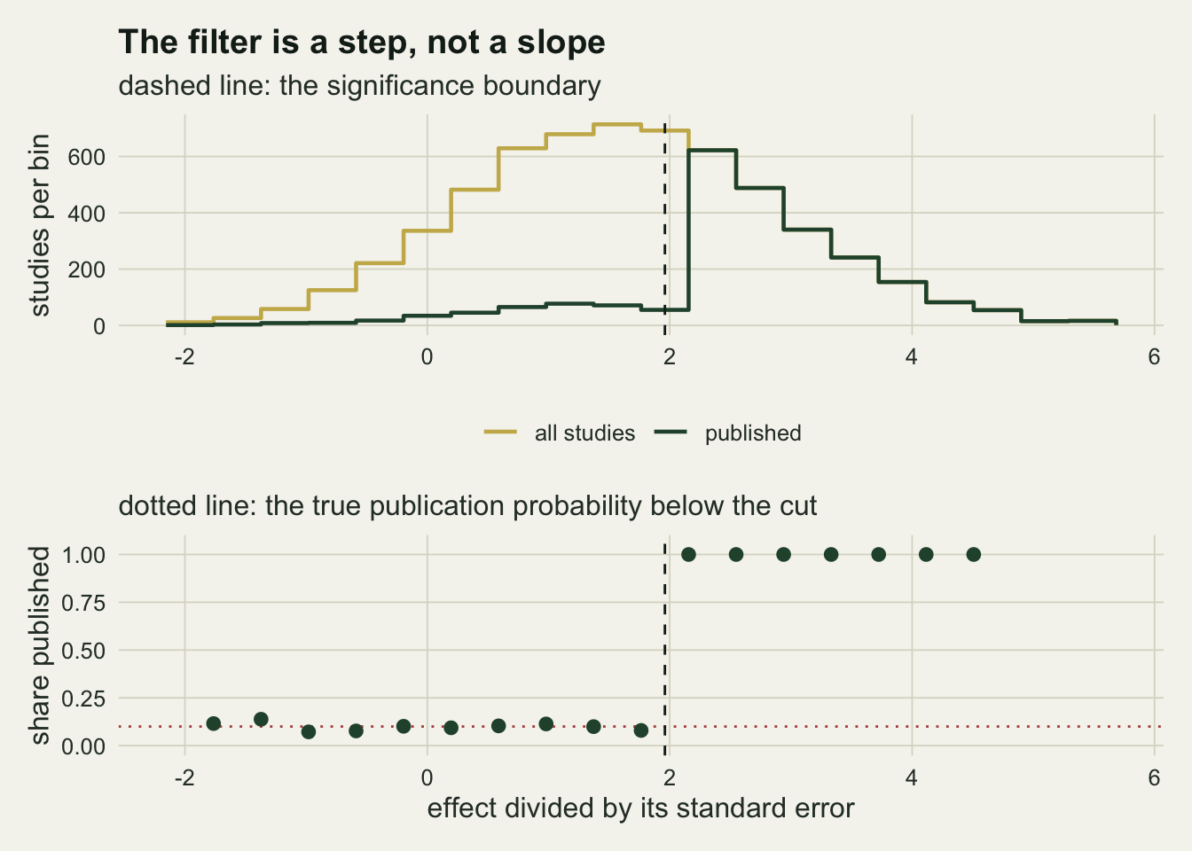
That step is the whole identification argument. The height of the jump is w, and a sample of published studies contains it as long as some of them fall on the low side of the cut.
The selection mechanism belongs in the denominator
Write \(s_i = \sqrt{v_i + \tau^2}\) for the marginal standard deviation of study \(i\), and \(z_c\) for the critical value. A published study contributes its ordinary random-effects density, times the weight its own p value earns, divided by the average weight over everything the study could have produced:
\[ \ell_i(\mu, \tau^2, w) = \log \phi\!\left(\frac{y_i - \mu}{s_i}\right) - \log s_i + \log(w)\,1\{z_i \le z_c\} - \log\!\big(P_i + w(1 - P_i)\big), \qquad P_i = 1 - \Phi\!\left(\frac{z_c\sqrt{v_i} - \mu}{s_i}\right) \]
\(P_i\) is the chance that this study would have been significant, so \(P_i + w(1 - P_i)\) is its chance of being published at all. The third term is the normalising constant, and it is what separates a selection model from a patch applied afterwards. Dropping the second and third terms gives back the ordinary random-effects likelihood, and that is the naive estimator every sweep below compares against.
## par = (mu, tau2, w); tau2 >= 0 and w in (0, 1] are BOX bounds, not transforms,
## so a boundary maximum is reported as one instead of being pushed to infinity
nll <- function(p, y, se, sel = TRUE) {
  mu <- p[1]; s <- sqrt(se^2 + p[2])
  ll <- dnorm(y, mu, s, log = TRUE)
  if (sel) {
    w <- p[3]; ll <- ll + ifelse(y / se > CRIT, 0, log(w))
    Ps <- pnorm((CRIT * se - mu) / s, lower.tail = FALSE)
    ll <- ll - log(Ps + w * (1 - Ps))
  }
  if (!all(is.finite(ll))) 1e10 else -sum(ll)
}

## standard errors from the Hessian over the free parameters only
par_se <- function(p, y, se, sel, free) {
  fn <- function(q) { pp <- p; pp[free] <- q; nll(pp, y, se, sel) }
  q <- p[free]; h <- pmax(1e-4, 1e-4 * abs(q))
  m <- length(q); hess <- matrix(0, m, m)
  for (i in 1:m) for (j in i:m) {
    e1 <- e2 <- numeric(m); e1[i] <- h[i]; e2[j] <- h[j]
    hess[i, j] <- hess[j, i] <- (fn(q + e1 + e2) - fn(q + e1 - e2) -
      fn(q - e1 + e2) + fn(q - e1 - e2)) / (4 * h[i] * h[j])
  }
  vc <- try(solve(hess), silent = TRUE)
  if (inherits(vc, "try-error")) return(rep(NA_real_, m))
  dg <- diag(vc); dg[!is.finite(dg) | dg <= 0] <- NA_real_; sqrt(dg)
}

## THREE starts for both fits: see the multistart experiment below
sel_starts <- function(y) list(c(mean(y), var(y), .3), c(min(y), .01, .05),
                               c(mean(y) - .2, .05, .5))
fit <- function(y, se, sel = TRUE, starts = NULL) {
  lo <- c(-10, 0, 1e-6); up <- c(10, 25, 1); np <- if (sel) 3 else 2
  if (is.null(starts)) starts <- if (sel) sel_starts(y) else
    list(c(mean(y), var(y)), c(mean(y), .01), c(min(y), .05))
  best <- NULL
  for (st in starts) {  # keep the lowest NLL of the three
    o <- try(optim(st[1:np], nll, y = y, se = se, sel = sel, method = "L-BFGS-B",
                   lower = lo[1:np], upper = up[1:np],
                   control = list(factr = 1e7, maxit = 500)), silent = TRUE)
    if (!inherits(o, "try-error") && is.finite(o$value) &&
        (is.null(best) || o$value < best$value)) best <- o
  }
  if (is.null(best)) return(list(mu = NA, tau2 = NA, w = NA, se = NA,
                                 se_w = NA, val = NA, code = NA, conv = FALSE))
  p <- best$par
  free <- c(TRUE, p[2] > 1e-8)            # tau2 = 0 is a legitimate maximum
  wbad <- if (sel) p[3] < 1e-4 || p[3] > 0.99999 else FALSE
  if (sel) free <- c(free, !wbad && p[3] < 0.999)
  s <- rep(NA_real_, np); s[free] <- par_se(p, y, se, sel, which(free))
  list(mu = p[1], tau2 = p[2], w = if (sel) p[3] else 1, se = s[1],
       se_w = if (sel) s[3] else NA_real_, val = best$value,
       code = best$convergence,
       conv = best$convergence == 0 && !wbad && is.finite(s[1]))
}

fit_scene <- fit(scene$y, scene$se, TRUE); naive_scene <- fit(scene$y, scene$se, FALSE)
print(round(c(mu = fit_scene$mu, tau = sqrt(fit_scene$tau2), w = fit_scene$w,
              se_mu = fit_scene$se, se_w = fit_scene$se_w,
              naive = naive_scene$mu, pooled = pooled_scene), 4))
mu tau w se_mu se_w naive pooled
0.3815 0.0931 0.1778 0.0806 0.1415 0.4880 0.4872 On the twenty-three study synthesis the selection fit returns 0.382 with a standard error of 0.081, against 0.488 from the same likelihood with the selection terms dropped and a truth of 0.30. It puts the publication probability for a non-significant study at 0.178, with a standard error of 0.142: the correction moves the estimate a long way while the parameter driving it is barely pinned down at this size. The inverse-variance pool of the same data, 0.487, differs from the naive random-effects fit by less than a thousandth here, but the two are different estimators and only the second is the one being swept below. One dataset proves nothing, so the next check is a literature large enough that sampling noise is not an explanation.
n_val <- 3000
set.seed(4021)
big_sel <- gen(n_val, mu_true, 0.20, w_true)
big_all <- gen(n_val, mu_true, 0.20, 1.00)
v_sel   <- fit(big_sel$y, big_sel$se, TRUE)
v_naive <- fit(big_sel$y, big_sel$se, FALSE)
v_none  <- fit(big_all$y, big_all$se, TRUE)
w_none_z <- (1 - v_none$w) / v_none$se_w
print(round(rbind(
  selection_model_on_filtered   = c(v_sel$mu, sqrt(v_sel$tau2), v_sel$w, v_sel$se_w),
  naive_model_on_filtered       = c(v_naive$mu, sqrt(v_naive$tau2), NA, NA),
  selection_model_on_unfiltered = c(v_none$mu, sqrt(v_none$tau2), v_none$w,
                                    v_none$se_w)), 4))
[,1] [,2] [,3] [,4]
selection_model_on_filtered 0.3008 0.1927 0.1042 0.0082
naive_model_on_filtered 0.5004 0.1169 NA NA
selection_model_on_unfiltered 0.2885 0.1992 0.9578 0.0611With 3000 published studies the selection model returns 0.3008 for a mean of 0.30 and 0.1042 for a publication probability of 0.10, while the naive random-effects fit on the same data returns 0.5004. Run on data with no filter at all, the same model puts the publication probability at 0.9578 with a standard error of 0.0611, so the boundary value of one, where it belongs, sits 0.69 standard errors away. That third row is the weakest of the three and it is the one to read with its uncertainty attached: on unfiltered data w is estimated loosely, and loosely near one is all the check can ask for.
This is the point where the comparison with the truncated parasite burdens post matters. There the same trick, a selection probability in the denominator, is used to correct counts truncated by host death, and the parameter that defines the truncation cannot be estimated: its profile likelihood is monotone, with no interior maximum, so the data prefer the smallest cut compatible with what was observed. Here the parameter is estimable, because the cut is not at the edge of the data but inside it, and the density of published effects has a visible step there. The same likelihood template gives an identified parameter in one problem and an unidentified one in the other, and the difference is where the cut falls relative to the data.
One start is not an optimum
Three parameters, two of them with a boundary in play, is exactly the geometry where a single call to optim stops somewhere that is not the maximum and reports convergence == 0 while doing it. Fitting each simulated literature from one start and from three, and keeping the lowest negative log-likelihood, measures how often that happens and what it costs.
gap_cut <- 0.10
compare_starts <- function(K, mu, tau, w, nsim, seed) {
  set.seed(seed)
  out <- t(vapply(seq_len(nsim), function(i) {
    d <- gen(K, mu, tau, w); ss <- sel_starts(d$y)
    one <- fit(d$y, d$se, TRUE, ss[1]); three <- fit(d$y, d$se, TRUE, ss)
    c(one$val, one$mu, three$val, three$mu, three$code)
  }, numeric(5)))
  worse <- out[, 1] - out[, 3] > 1e-6
  gap <- abs(out[, 2] - out[, 4])[worse]
  c(K = K, mu = mu, nsim = nsim, conv = mean(out[, 5] == 0), frac = mean(worse),
    frac_se = sqrt(mean(worse) * (1 - mean(worse)) / nsim), n_worse = sum(worse),
    med_gap = median(gap), n_small = sum(gap <= gap_cut), max_gap = max(gap))
}
starts_tab <- rbind(compare_starts(20, 0.30, tau_true, w_true, n_start, 90811),
                    compare_starts(8,  0.50, tau_true, w_true, n_start, 55117))
print(round(starts_tab, 4))
K mu nsim conv frac frac_se n_worse med_gap n_small max_gap
[1,] 20 0.3 400 0.9325 0.065 0.0123 26 0.0002 26 0.0134
[2,] 8 0.5 400 0.9625 0.030 0.0085 12 0.0085 10 2.0903Each cell is 400 simulated literatures, and optim reported convergence on the three-start fit in 93.2 and 96.2 per cent of them. At twenty studies with severe selection the single start stops above the three-start optimum in 6.5 per cent of fits, with a Monte Carlo standard error of 1.2 points, and it costs almost nothing: over those 26 fits the largest shift in the estimated mean is 0.013. Frequency is not severity. On the harder cell, eight studies of a large true effect, the single start is worse less often, 3.0 per cent, or 12 fits, and the damage sits in the tail rather than in the body: 10 of those shift the estimated mean by less than 0.10, the median shift is 0.0085, and one single replicate shifts it by 2.09, several times the effect being estimated. A rare fit that is wrong by more than the effect is not a rounding problem. Every number below therefore comes from three starts, for the naive fit as well as for the selection model.
The break-even is a surface, not a number
The advice to fit a selection model once there are more than about ten studies is a statement about one cell. What follows sweeps the true mean across three values, holding the between-study standard deviation and the publication probability fixed, and reports for each cell the share of usable fits, the root mean squared error of both estimators, their ratio, and the coverage of the nominal interval.
A fit counts as usable when optim converged, the publication probability did not end on either box boundary, and the Hessian over the free parameters could be inverted. Which fits enter which summary matters more than it looks. The naive columns are taken over every literature where the naive fit was usable; the ratio compares the two estimators on the literatures where both were usable, so it is like for like; and the practitioner column, which uses the selection estimate when it is available and the naive one when it is not, is compared against the naive column over the same set. The replication was fixed before any of this was run: 350 simulated literatures per cell.
Ks <- c(5, 8, 12, 20, 40); mus <- c(0, 0.30, 0.50)

ratio_mcse <- function(es, en, B = 400) sd(replicate(B, {
  i <- sample.int(length(es), length(es), TRUE)
  sqrt(mean(es[i]^2)) / sqrt(mean(en[i]^2)) }))

run_cell <- function(K, mu, tau, w, nsim) {
  out <- matrix(NA_real_, nsim, 8)
  for (i in seq_len(nsim)) {
    d  <- gen(K, mu, tau, w)
    fn <- fit(d$y, d$se, FALSE); fs <- fit(d$y, d$se, TRUE)
    out[i, ] <- c(fn$mu, fn$se, fn$conv, fs$mu, fs$se, fs$conv,
                  ifelse(fs$conv, fs$mu, fn$mu), fs$w)  # 7: practitioner fallback
  }
  okn <- out[, 3] == 1 & is.finite(out[, 2])
  oks <- out[, 6] == 1 & is.finite(out[, 5]); keep <- okn & oks
  en <- out[okn, 1] - mu; ef <- out[okn, 7] - mu        # naive set
  ep <- out[keep, 1] - mu; es <- out[keep, 4] - mu      # paired set
  cn <- abs(out[okn, 1] - mu) <= 1.96 * out[okn, 2]
  cs <- abs(out[oks, 4] - mu) <= 1.96 * out[oks, 5]
  data.frame(K = K, mu_true = mu, conv = mean(oks),
    conv_se = sqrt(mean(oks) * (1 - mean(oks)) / nsim),
    bias_n = mean(en), bias_p = mean(ep), bias_s = mean(es),
    bias_s_se = sd(es) / sqrt(length(es)), n_s = length(es), n_n = length(en),
    rmse_n = sqrt(mean(en^2)), rmse_p = sqrt(mean(ep^2)), rmse_s = sqrt(mean(es^2)),
    ratio = sqrt(mean(es^2)) / sqrt(mean(ep^2)), ratio_se = ratio_mcse(es, ep),
    fb_ratio = sqrt(mean(ef^2)) / sqrt(mean(en^2)), fb_se = ratio_mcse(ef, en),
    se_n = mean(out[okn, 2]), se_s = mean(out[oks, 5]),
    w_cor = cor(out[oks, 8], out[oks, 4] - mu), cov_n = mean(cn),
    cov_n_se = sd(cn) / sqrt(length(cn)), cov_s = mean(cs), n_cov_s = length(cs),
    cov_s_se = sd(cs) / sqrt(length(cs)))
}

set.seed(20826)
surface <- do.call(rbind, lapply(mus, function(mu)
  do.call(rbind, lapply(Ks, function(K) run_cell(K, mu, tau_true, w_true, n_surface)))))
## print a subset under short names so the table fits the page width
tab_short <- function(d, cols, nm) { d <- d[, cols]; names(d) <- nm
                                     format(d, digits = 3) }
print(tab_short(surface,
  c("K", "mu_true", "conv", "bias_n", "rmse_n", "rmse_p", "rmse_s", "ratio",
    "ratio_se", "fb_ratio", "cov_n", "cov_s"),
  c("K", "mu", "conv", "biasN", "rmseN", "rmseP", "rmseS", "ratio", "ratSE",
    "fbRat", "covN", "covS")))
K mu conv biasN rmseN rmseP rmseS ratio ratSE fbRat covN covS
1 5 0.0 0.737 0.1791 0.236 0.2437 0.1521 0.624 0.0268 0.718 0.6227 0.953
2 8 0.0 0.834 0.1821 0.213 0.2137 0.1228 0.575 0.0236 0.663 0.5895 0.955
3 12 0.0 0.877 0.1654 0.190 0.1895 0.0956 0.505 0.0206 0.592 0.5401 0.938
4 20 0.0 0.880 0.1736 0.189 0.1903 0.0793 0.417 0.0170 0.507 0.3313 0.935
5 40 0.0 0.889 0.1733 0.181 0.1815 0.0560 0.309 0.0145 0.442 0.0973 0.929
6 5 0.3 0.503 0.1857 0.208 0.1716 0.1779 1.037 0.1018 1.013 0.4771 0.949
7 8 0.3 0.674 0.1863 0.197 0.1835 0.1460 0.795 0.0401 0.886 0.2687 0.958
8 12 0.3 0.823 0.1803 0.190 0.1838 0.1470 0.800 0.0426 0.850 0.1567 0.885
9 20 0.3 0.909 0.1811 0.186 0.1853 0.1225 0.661 0.0360 0.703 0.0358 0.893
10 40 0.3 0.937 0.1806 0.183 0.1837 0.0942 0.513 0.0228 0.554 0.0000 0.860
11 5 0.5 0.146 0.1051 0.140 0.0634 0.2043 3.222 0.5685 1.134 0.8075 0.961
12 8 0.5 0.303 0.0963 0.118 0.0966 0.1878 1.945 0.4055 1.245 0.7880 0.981
13 12 0.5 0.449 0.1005 0.116 0.0968 0.1324 1.367 0.1097 1.124 0.6542 0.943
14 20 0.5 0.623 0.1032 0.113 0.1036 0.1046 1.010 0.1194 1.005 0.3625 0.959
15 40 0.5 0.803 0.1034 0.109 0.1073 0.0798 0.744 0.0577 0.809 0.1369 0.890nominal <- 0.95
cov_s_lo <- min(surface$cov_s); cov_hi <- surface[which.max(surface$cov_s), ]
rse_lo <- min(surface$ratio_se); rse_hi <- surface[which.max(surface$ratio_se), ]
fb_gap <- surface[which.max(abs(surface$fb_ratio - surface$ratio)), ]
at <- function(mu, K) surface[surface$mu_true == mu & surface$K == K, ]
r_null_5 <- at(0, 5); r_mid_5 <- at(0.30, 5); r_mid_8 <- at(0.30, 8)
r_mid_40 <- at(0.30, 40); r_big_5 <- at(0.50, 5); r_big_8 <- at(0.50, 8)
r_big_20 <- at(0.50, 20); r_big_40 <- at(0.50, 40)At a true mean of zero the selection model is already ahead at the smallest size tried: an error ratio of 0.624 with a Monte Carlo error of 0.027 at 5 studies. At a true mean of 0.30 the ratio at the same size is 1.037 plus or minus 0.102, a bar that covers a tie, and it drops below one by 8 studies (0.795 plus or minus 0.040). At a true mean of 0.50 the ratio is 1.945 plus or minus 0.405 at 8 studies and 1.010 plus or minus 0.119 at 20, an error bar that reaches under one, and only at 40 studies does it clear the tie, at 0.744 plus or minus 0.058. The point estimates cross below five studies at one end of that axis and between 20 and 40 at the other, and at 20 studies the cell on its own cannot be told from a tie.
That Monte Carlo error is not uniform, and the cells the argument leans on hardest are the imprecise ones. It runs from 0.014 in the best behaved cell to 0.568 at a true mean of 0.50 with 5 studies, where the ratio rests on the 48 literatures in which both fits were usable rather than on all 350. Those cells carry the claim that the two estimators tie, which an imprecise ratio supports rather than undermines; they do not carry any claim about where exactly the crossing falls, and none is made.
The mechanism is visible in the bias column. Selection can only distort what it removes, and when the true effect is large relative to the standard errors most studies clear the boundary on their own. The naive bias at 5 studies is 0.105 when the true mean is 0.50, against 0.179 when the true mean is zero. There is less to correct, and the correction still costs its parameter. That column repays a second look: over the subset where the selection fit also converged, the same naive bias in that corner reads 0.015, about a seventh of the unconditional value, because those are the literatures that happened to contain unselected studies. A summary of one estimator conditioned on the success of the other is a self-selected summary, which is the fault this section is about to name.
The same shortage of unselected studies wrecks the fitting. Usable fits fall to 0.146 of 350 in that corner, against 0.737 at a true mean of zero. A break-even quoted without its convergence rate is quoting the performance of the fits that happened to work. The practitioner column, which falls back on the naive estimate whenever the selection fit fails, is the honest one, and on this grid it moves no crossing: at a true mean of 0.30 it reads 1.013 plus or minus 0.037 at 5 studies and 0.886 plus or minus 0.022 at 8, the same side of one as the conditional column at both, though at five studies both bars still cover a tie. What it changes is the size of the prize. Everywhere in this grid the practitioner ratio lands on the same side of one as the conditional ratio and nearer to one, and where convergence collapses the two are far apart: at a true mean of 0.50 with 5 studies the conditional ratio is 3.222 against a practitioner ratio of 1.134, because a practitioner who falls back is mostly reporting the naive estimate.
surface$effect <- factor(sprintf("true mean %.2f", surface$mu_true))
ggplot(surface, aes(K, ratio, colour = effect)) +
  geom_hline(yintercept = 1, linetype = "dashed", colour = te_ink, linewidth = 0.5) +
  geom_errorbar(aes(ymin = ratio - ratio_se, ymax = ratio + ratio_se),
                width = 0.04, linewidth = 0.5) +
  geom_line(linewidth = 0.9) + geom_point(size = 2.3) +
  scale_x_log10(breaks = Ks) +
  scale_colour_manual(values = c(te_forest, te_gold, te_rust), name = NULL) +
  labs(x = "published studies", y = "error ratio, selection over naive",
       title = "The break-even is a surface, not a number",
       subtitle = "dashed line: the two estimators tie") +
  theme_datasheet() + theme(legend.position = "bottom")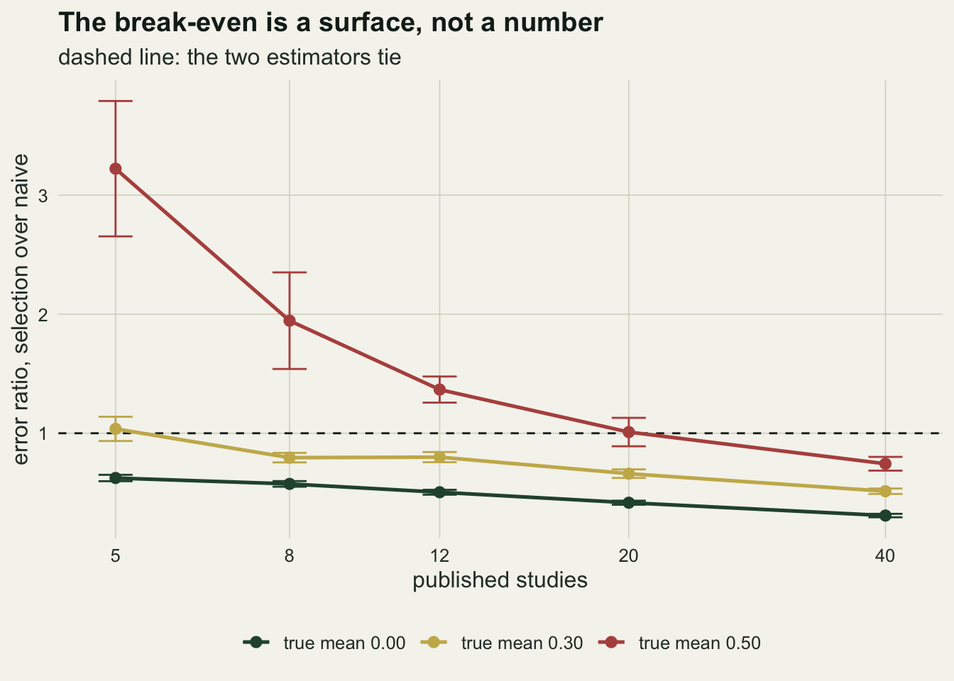
Coverage and the point estimate do not agree
The error ratio is one axis. The interval is another, and it ranks the two estimators the other way round. The two coverage columns are not over the same fits: the naive one is over every literature where the naive fit was usable, the selection one over every literature where the selection fit was usable, and where convergence collapses that second set is much the smaller, 51 fits against 322 in the worst corner.
mid_row <- surface[surface$mu_true == mus[2], ]
cov_dat <- rbind(
  data.frame(K = mid_row$K, cov = mid_row$cov_n, se = mid_row$cov_n_se, fit = "naive"),
  data.frame(K = mid_row$K, cov = mid_row$cov_s, se = mid_row$cov_s_se,
             fit = "selection model"))
ggplot(cov_dat, aes(K, cov, colour = fit)) +
  geom_hline(yintercept = nominal, linetype = "dotted",
             colour = te_ink, linewidth = 0.5) +
  geom_errorbar(aes(ymin = cov - se, ymax = cov + se), width = 0.04, linewidth = 0.5) +
  geom_line(linewidth = 0.9) + geom_point(size = 2.3) +
  scale_x_log10(breaks = Ks) + scale_y_continuous(limits = c(0, 1)) +
  scale_colour_manual(values = c(te_rust, te_forest), name = NULL) +
  labs(x = "published studies", y = "coverage of the nominal interval",
       title = "On the interval there is no break-even",
       subtitle = "dotted line: the nominal level") +
  theme_datasheet() + theme(legend.position = "bottom")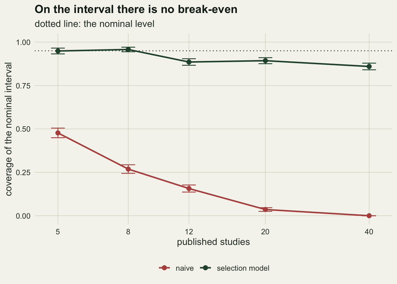
At a true mean of 0.30 the naive interval covers the truth in 0.477 of fits at 5 studies (Monte Carlo error 0.028) and in 0.000 of 303 fits at 40: not one interval in the largest cell contained the true effect. The selection model covers in 0.949 and 0.860 of fits at the same two sizes, the latter with a Monte Carlo error of 0.019, which is 9 points below the nominal 0.95.
The two axes disagree openly. On the interval the selection model is ahead everywhere, including the cells where its point estimate is worse, and the gap widens with the number of studies because more studies make the naive interval narrower without moving it back towards the truth. On squared error it is behind until somewhere between 5 and 8 studies at a moderate effect, and somewhere between 20 and 40 at a large one, where only the larger of those two cells separates from a tie. Nothing resolves that contradiction, and a review that reports both numbers has said more than one that picks a winner.
The price of correcting a bias that was not there
A selection model is fitted because the funnel leans. Funnels lean for several reasons, so the case worth measuring is the one where the analyst fits the model and there was no filter at all. The publication probability is then one, the model is still correct, and the extra parameter sits on its boundary.
K_nosel <- c(5, 12, 20, 40, 60)
set.seed(51771)
nosel <- do.call(rbind, lapply(K_nosel, function(K)
  run_cell(K, mu_true, tau_true, 1.0, n_nosel)))
print(tab_short(nosel,
  c("K", "conv", "bias_n", "bias_s", "bias_s_se", "rmse_n", "rmse_s", "ratio",
    "fb_ratio", "cov_n", "cov_s"),
  c("K", "conv", "biasN", "biasS", "biasSse", "rmseN", "rmseS", "ratio",
    "fbRat", "covN", "covS")))
K conv biasN biasS biasSse rmseN rmseS ratio fbRat covN covS
1 5 0.470 -0.001977 -0.0932 0.01115 0.1235 0.1565 1.44 1.18 0.880 0.957
2 12 0.410 -0.000796 -0.0729 0.00870 0.0759 0.1164 1.55 1.25 0.916 0.878
3 20 0.463 -0.004264 -0.0632 0.00599 0.0580 0.0913 1.49 1.27 0.918 0.899
4 40 0.453 0.001023 -0.0411 0.00443 0.0406 0.0641 1.76 1.33 0.952 0.926
5 60 0.417 -0.001242 -0.0308 0.00366 0.0311 0.0492 1.68 1.30 0.958 0.920ns_5 <- nosel[nosel$K == 5, ]; ns_60 <- nosel[nosel$K == 60, ]
conv_lo <- min(nosel$conv); conv_hi <- max(nosel$conv)
ratio_lo <- min(nosel$ratio); ratio_hi <- max(nosel$ratio)
fb_lo <- min(nosel$fb_ratio); fb_hi <- max(nosel$fb_ratio)
ncov_lo <- min(nosel$cov_s); ncov_hi <- max(nosel$cov_s) # no-selection sweep
bias_z <- abs(ns_60$bias_s) / ns_60$bias_s_se; se_infl <- ns_60$se_s / ns_60$se_nThree things come out of that table and none of them is about variance. The share of usable fits sits between 0.410 and 0.470 and does not improve with the number of studies: at 60 studies it is still 0.417, with a Monte Carlo error of 0.028, so more than half of the fits cannot be reported at all. That is the real bill. The estimator is not noisy, it is unavailable.
The fits that do come back are biased downwards, and the bias does not vanish. It is -0.093 at 5 studies and -0.031 at 60, the latter with a Monte Carlo standard error of 0.0037, so it is 8 standard errors from zero on the 111 of 300 replicates where both fits were usable, the set the bias column is taken over. Convergence is itself a selection: a fit is kept when the publication probability comes back below one, which keeps the samples in which the model found a filter that did not exist. That is measurable rather than merely arguable. Across the wider set of 125 replicates whose selection fit was usable at 60 studies, the share the convergence column counts, the fitted publication probability and the error in the estimated mean correlate at 0.69: the fits that report the most selection are the fits that are furthest below the truth. Root mean squared error is inflated by a factor between 1.44 and 1.76 among the fits that come back, and between 1.18 and 1.33 for an analyst who falls back on the naive fit when they do not, and neither factor shrinks with the number of studies.
The interval, in contrast, survives: coverage of the selection model’s interval runs from 0.878 to 0.957 against the nominal 0.95, with none of the collapse the point estimate shows. The reason is that the standard error inflates along with the error. At 60 studies the selection model’s mean standard error is 0.0499 against 0.0329 for the naive fit, a factor of 1.52, close to the 1.68 by which its actual error is inflated. So the cost of a needless selection model is not a wider interval. It is that more than half of the analyses have no result at all, and the ones that do are pulled towards a correction that was never called for.
What to report
Report the publication probability with its own uncertainty, not only the corrected mean. A fit that puts it at a tenth is claiming that nine in ten null results were never written up, which is a strong claim about a field and should be argued rather than tabled quietly. On twenty-three studies that parameter came with a standard error most of the way to its own size, and a corrected mean quoted without it hides how little the data said. Report as well the number of studies that fell on the low side of the significance boundary: that count, not the total, is what identifies the selection parameter, and a synthesis in which almost every published study is significant carries almost no information about the filter, whatever its size.
Say whether the fit converged and what was done when it did not. Falling back on the uncorrected estimate is a defensible choice and it changes the operating characteristics, as the practitioner column above shows. Silently dropping the failures is not defensible, because the failures are not a random subset: the fits that survive are the ones that found the most selection.
Give the corrected estimate next to the uncorrected one and let the reader see the size of the correction. If the two agree, the selection model has cost nothing but a parameter. If they disagree by more than the interval, that gap is the finding, and it deserves the sensitivity analysis that Copas and Shi (2000) argue for: vary the assumed selection rather than trusting the fitted one. In reviews with few studies and a pooled effect that is large relative to the standard errors, treat the whole exercise as a sensitivity analysis, because that is the corner where the numbers above say the correction is at best a tie on squared error while it is already worth having on the interval.
Honest limits
The sampling variances are treated as known. Real standardised mean differences carry an estimated variance that is correlated with the effect itself, which is a known source of funnel asymmetry with nothing to do with publication, and it is absent from every simulation here. Nothing in this post speaks to how the estimator behaves once that correlation is present.
The model is true at the point of fitting, and that is the largest limit in the post. A hard cutpoint at a one-sided p of 0.025 is a caricature of how journals and authors behave: real selection is graded, responds to effect size as well as to significance, and has more than one threshold. Every number here is therefore a best case. Vevea and Hedges (1995) allow several intervals of the p value with their own weights, and Carter et al. (2019) compare the resulting estimators under mechanisms that are deliberately not the fitted one; both show that the guarantees soften under misspecification.
The standard errors come from inverting a numerical Hessian over the non-boundary parameters, and they are mildly anti-conservative where it matters. Coverage of the selection model’s interval runs from 0.860 to 0.981 across the surface against a nominal 0.95, and at a moderate true effect it sits below the target at every size past eight studies. The cell that reaches 0.981 is one where only 0.303 of fits survive, so its coverage describes a small self-selected group. The interval is in a much better place than the naive one, but it is not the advertised level and reporting it as exact would be wrong.
Every quantity in the table is conditional on something. Where the share of usable fits is 0.146, as it is for a large true effect with five studies, the conditional error ratio describes a small and self-selected subset of the simulated literatures, which is why the practitioner column exists and why it is the one to quote to a reader who intends to actually fit this. The two columns never disagree about which estimator wins in this grid, but they disagree about the margin by as much as 2.09.
The generator keeps the first K published studies from a pool rather than a random sample of everything ever published, which is not quite a random sample of the published literature. With a large pool the difference is small, but it is a departure from the way meta-analytic samples are usually described. Jennions and Moller (2002) and Nakagawa et al. (2022) give the ecological context these simulations are standing in for: how common asymmetry is in ecological and evolutionary syntheses, and which corrections behave sensibly when it is found.
References
Iyengar S, Greenhouse JB 1988 Statistical Science 3(1) (10.1214/ss/1177013012)
Hedges LV 1992 Statistical Science 7(2) (10.1214/ss/1177011364)
Vevea JL, Hedges LV 1995 Psychometrika 60(3):419-435 (10.1007/BF02294384)
Copas J, Shi JQ 2000 Biostatistics 1(3):247-262 (10.1093/biostatistics/1.3.247)
Jennions MD, Moller AP 2002 Biological Reviews 77(2):211-222 (10.1017/S1464793101005875)
Carter EC, Schonbrodt FD, Gervais WM, Hilgard J 2019 Advances in Methods and Practices in Psychological Science 2(2):115-144 (10.1177/2515245919847196)
Nakagawa S, Lagisz M, Jennions MD, Koricheva J, Noble DWA, Parker TH, Sanchez-Tojar A, Yang Y, O’Dea RE 2022 Methods in Ecology and Evolution 13(1):4-21 (10.1111/2041-210X.13724)