library(ggplot2)
library(patchwork)

te_paper  <- "#f5f4ee"
te_ink    <- "#16241d"
te_body   <- "#2c3a31"
te_forest <- "#275139"
te_rust   <- "#b5534e"
te_gold   <- "#c9b458"
te_line   <- "#dad9ca"

theme_datasheet <- function() {
  theme_minimal(base_size = 12) +
    theme(plot.background  = element_rect(fill = te_paper, colour = NA),
          panel.background = element_rect(fill = te_paper, colour = NA),
          panel.grid.major = element_line(colour = te_line, linewidth = 0.3),
          panel.grid.minor = element_blank(),
          text             = element_text(colour = te_body),
          plot.title       = element_text(colour = te_ink, face = "bold"),
          plot.subtitle    = element_text(colour = te_body),
          axis.text        = element_text(colour = te_body))
}PET-PEESE and publication bias under heterogeneity
R
meta-analysis
publication bias
simulation
ecology tutorial
PET-PEESE removes publication bias that grows with the standard error, not a significance filter on studies that differ by site. Measured in base R simulations.
A review of grazing exclosures and plant species richness has thirty studies, each giving a standardised mean difference between fenced and grazed plots. The funnel plot leans: the small studies sit to the right. Egger’s test is run, and a reviewer asks for the regression correction that the ecological guidance now points to. Nakagawa and colleagues (2022) set out Egger-type meta-regression with the standard error as a moderator as the workhorse for ecological and evolutionary syntheses, and the specific estimator most people reach for is PET-PEESE: regress the effect sizes on their standard errors, read the intercept as the effect of a study with no sampling error, and switch to a regression on the variance when that intercept is clearly positive (Stanley and Doucouliagos 2014).
That estimator rests on one assumption about the published literature: that the expected effect, given the standard error, is a straight line (or a parabola) that passes through the true mean at a standard error of zero. Whether selection breaks that assumption depends on what kind of selection it is, and ecological syntheses contain two kinds. A journal or an author can drop a whole study that came out non-significant. That is a filter between studies. An author who measured richness, cover, biomass and a diversity index can report the one that moved most. That is selection within a study, and the study is published either way.
This post measures PET, PEESE and the conditional PET-PEESE rule under both. The failure it leads with is not new: Stanley (2017) reported that PET-PEESE performs poorly when heterogeneity is very high, and Carter and colleagues (2019) found in a large comparison that no correction won across conditions. What is shown here is where that failure comes from in a form that can be written down, why the within-study case is repaired by construction, and how rarely Egger’s test would have triggered the correction in either case. The contrast between the two kinds of selection is assembled from those sources rather than discovered here.
The post sits between two existing ones. Checking for publication bias builds the funnel plot, Egger’s test and trim-and-fill, and says in its limits, in prose, that trim-and-fill can add studies that never existed when the real cause is heterogeneity; it fits no regression correction and measures no heterogeneity effect. Selection models for publication bias corrects by writing the filter into the likelihood and prices that model when there was no filter. Neither fits PET or PEESE, and neither has selection among the responses of a single study. Dependent effect sizes in meta-analysis treats the study with several responses, but there every response is reported; here only the largest is.
Three regressions, a rule and a test
Every estimator below uses known sampling variances, so the only thing an estimator has to get right is the treatment of selection. Random effects is DerSimonian and Laird’s moment estimator of tau-squared followed by an inverse variance weighted mean (DerSimonian and Laird 1986). PET is a weighted least squares regression of the effect on its standard error with weights one over the variance, and its intercept is the estimate. PEESE is the same regression on the variance instead of the standard error. Both are fitted as unrestricted weighted least squares, which is how Stanley and Doucouliagos fit them: the residual variance is estimated, not fixed at one.
The conditional rule uses PET unless PET’s intercept is significantly positive, and then uses PEESE. Stanley (2017) recommends switching when a one-sided test of a non-positive intercept rejects at 0.10, and that is the main rule here. Two variants are carried for comparison: a one-sided test at 0.05, the stricter version, and a two-sided test at 0.10, which also switches when the intercept is significantly negative. The two-sided variant is not a published PET-PEESE rule; it is included to show what that extra switch does. Trim-and-fill is the L0 function from the funnel post, with the filled set pooled by random effects. A multilevel version of PET, in the spirit of Nakagawa and colleagues, is added as a random effects meta-regression with a moment estimate of the residual tau-squared; with one effect per study there is no second level to add, so this is the multilevel model reduced to what the data can carry.
dl_fit <- function(y, v) {
  w <- 1 / v; k <- length(y); m_fe <- sum(w * y) / sum(w)
  q_stat <- sum(w * (y - m_fe)^2)
  tau2 <- max(0, (q_stat - (k - 1)) / (sum(w) - sum(w^2) / sum(w)))
  ws <- 1 / (v + tau2); est <- sum(ws * y) / sum(ws)
  c(est = est, se = sqrt(1 / sum(ws)), tau2 = tau2, q = q_stat)
}

# weighted least squares of y on x; residual variance estimated (unrestricted)
wls_fit <- function(y, x, w) {
  k <- length(y); sw <- sum(w); xm <- sum(w * x) / sw; ym <- sum(w * y) / sw
  sxx <- sum(w * (x - xm)^2); b <- sum(w * (x - xm) * (y - ym)) / sxx
  a <- ym - b * xm; rss <- sum(w * (y - a - b * x)^2)
  s2 <- rss / (k - 2)
  c(a = a, se_a = sqrt(s2 * (1 / sw + xm^2 / sxx)), b = b,
    se_b = sqrt(s2 / sxx), rss = rss)
}

# PET as a random effects meta-regression: moment tau2 from the residual Q
pet_re <- function(y, se) {
  v <- se^2; k <- length(y); w0 <- 1 / v
  f0 <- wls_fit(y, se, w0)
  x_mat <- cbind(1, se)
  xtwx  <- crossprod(x_mat * w0, x_mat); xtw2x <- crossprod(x_mat * w0^2, x_mat)
  tr_p  <- sum(w0) - sum(diag(solve(xtwx, xtw2x)))
  tau2  <- max(0, (f0[["rss"]] - (k - 2)) / tr_p)
  w1 <- 1 / (v + tau2); sw <- sum(w1); xm <- sum(w1 * se) / sw
  sxx <- sum(w1 * (se - xm)^2)
  b <- sum(w1 * (se - xm) * (y - sum(w1 * y) / sw)) / sxx
  sum(w1 * y) / sw - b * xm
}

trimfill_l0 <- function(g, se) {
  v <- se^2; k <- length(g); wmean <- function(yy, vv) sum(yy / vv) / sum(1 / vv)
  mu0 <- wmean(g, v); side <- if (sum(sign(g - mu0)) >= 0) 1 else -1
  yy <- side * g; ord <- order(yy); k0 <- 0; k0o <- -1; mu_c <- mu0; it <- 0
  while (k0 != k0o && it < 100) {
    it <- it + 1; k0o <- k0
    keep <- if (k0 > 0) ord[1:(k - k0)] else ord
    mu_c <- wmean(g[keep], v[keep]); cen <- side * mu_c
    dd <- yy - cen; rk <- rank(abs(dd)); tn <- sum(rk[dd > 0])
    k0 <- max(0, round((4 * tn - k * (k + 1)) / (2 * k - 1)))
  }
  cen <- side * mu_c
  if (k0 > 0) {
    ex <- ord[(k - k0 + 1):k]
    ga <- c(g, side * (2 * cen - yy[ex])); sa <- c(se, se[ex])
  } else { ga <- g; sa <- se }
  dl_fit(ga, sa^2)[["est"]]
}

fit_all <- function(y, se) {
  k <- length(y); v <- se^2; qk <- qt(0.975, k - 2)
  re <- dl_fit(y, v)
  pet <- wls_fit(y, se, 1 / v); peese <- wls_fit(y, v, 1 / v)
  t_int <- pet[["a"]] / pet[["se_a"]]
  p_one <- pt(t_int, k - 2, lower.tail = FALSE)
  sw_10 <- p_one < 0.10      # Stanley (2017): one-sided test at 0.10
  sw_05 <- p_one < 0.05      # stricter one-sided version
  two_sided <- 2 * pt(abs(t_int), k - 2, lower.tail = FALSE) < 0.10  # not published
  egger <- 2 * pt(abs(pet[["b"]] / pet[["se_b"]]), k - 2, lower.tail = FALSE) < 0.10
  pp_est <- if (sw_10) peese else pet
  c(re = re[["est"]],
    re_lo = re[["est"]] - qnorm(0.975) * re[["se"]],
    re_hi = re[["est"]] + qnorm(0.975) * re[["se"]],
    pet = pet[["a"]], pet_lo = pet[["a"]] - qk * pet[["se_a"]],
    pet_hi = pet[["a"]] + qk * pet[["se_a"]],
    peese = peese[["a"]],
    pp1 = pp_est[["a"]], pp2 = if (sw_05) peese[["a"]] else pet[["a"]],
    pp3 = if (two_sided) peese[["a"]] else pet[["a"]],
    pp_lo = pp_est[["a"]] - qk * pp_est[["se_a"]],
    pp_hi = pp_est[["a"]] + qk * pp_est[["se_a"]],
    petre = pet_re(y, se), tf = trimfill_l0(y, se),
    i2 = max(0, (re[["q"]] - (k - 1)) / re[["q"]]),
    egger = egger, switch = sw_10)
}
Egger’s test and PET are the same regression. Dividing Egger’s model, effect over standard error regressed on precision, through by the precision gives PET with weights one over the variance: Egger’s intercept is PET’s slope and Egger’s slope is PET’s intercept, with identical t statistics. The test that tells an analyst to correct is therefore the slope of the correction itself, which matters later when its detection rate is measured. The check below fits both on one simulated synthesis.
z_crit <- qnorm(0.975)
n_min <- 5; n_max <- 60           # per arm sample sizes, uniform

# between study filter: significant positive studies always published,
# the rest with probability w_pub
draw_filter <- function(k, mu, tau, w_pub) {
  y <- se <- numeric(0)
  while (length(y) < k) {
    nb <- 4 * k
    s <- sqrt(2 / sample(n_min:n_max, nb, TRUE))
    yy <- rnorm(nb, mu, tau) + s * rnorm(nb)
    keep <- (yy / s > z_crit) | (runif(nb) < w_pub)
    y <- c(y, yy[keep]); se <- c(se, s[keep])
  }
  list(y = y[1:k], se = se[1:k])
}

# within study selection: m responses, equicorrelated errors rho, largest reported
draw_within <- function(k, mu, tau, m, rho) {
  s <- sqrt(2 / sample(n_min:n_max, k, TRUE))
  z <- sqrt(rho) * rnorm(k) + sqrt(1 - rho) * matrix(rnorm(k * m), k, m)
  list(y = rnorm(k, mu, tau) + s * apply(z, 1, max), se = s)
}

set.seed(318)
demo <- draw_filter(30, 0, 0.4, 0.2)
egger_lm <- summary(lm(I(demo$y / demo$se) ~ I(1 / demo$se)))$coefficients
pet_lm   <- summary(lm(demo$y ~ demo$se, weights = 1 / demo$se^2))$coefficients
id_gap <- max(abs(egger_lm[, "t value"] - rev(pet_lm[, "t value"])))
egger_lm; pet_lm
Estimate Std. Error t value Pr(>|t|)
(Intercept) -1.0371022 1.8459647 -0.5618213 0.5787077
I(1/demo$se) 0.6025141 0.4440273 1.3569304 0.1856426 Estimate Std. Error t value Pr(>|t|)
(Intercept) 0.6025141 0.4440273 1.3569304 0.1856426
demo$se -1.0371022 1.8459647 -0.5618213 0.5787077On that synthesis Egger’s intercept t is -0.5618 and PET’s slope t is -0.5618; the largest difference between the matching t statistics is below one in ten billion.
The design constants are fixed before any of the runs: per arm sample sizes from 5 to 60, a standard error of the square root of two over n, a filter that publishes every study significant and positive at the two-sided 0.05 boundary and each other study with probability 0.2 (or 1, for no selection), and four responses for the within-study case.
Two ways a literature leans
Before simulating anything, the expected published effect at a given standard error can be written down for both kinds of selection. For the within-study case it is a one line result. The reported response is the true study effect plus the standard error times the largest of four equicorrelated standard normals, and the largest of equicorrelated normals is the shared part plus the square root of one minus rho times the largest of four independent ones. So the expected effect is the mean plus a constant times the standard error. That is exactly PET’s model, whatever tau is, which means PET is unbiased there by construction and nothing in a simulation can show otherwise.
For the filter the expected published effect follows from a truncated normal. The observed effect is normal around the mean with variance tau-squared plus the sampling variance; the filter keeps everything above 1.96 standard errors and a fraction w of the rest. When tau is zero and the true mean is zero, the published effect is the standard error times a fixed truncated mean, again a line through zero, and PET is right. When tau is not zero, a study with a tiny standard error is still filtered: it is significant exactly when its own true effect is positive. At a standard error of zero the published mean is the mean of true effects among those published, not the true mean.
w_sel <- 0.2; rho_mid <- 0.5; m_resp <- 4
filter_bias <- function(se, mu, tau, w_pub) {
  s_tot <- sqrt(tau^2 + se^2); a_std <- (z_crit * se - mu) / s_tot
  p_up <- pnorm(a_std, lower.tail = FALSE)
  e_up <- mu * p_up + s_tot * dnorm(a_std)
  e_lo <- mu * (1 - p_up) - s_tot * dnorm(a_std)
  (e_up + w_pub * e_lo) / (p_up + w_pub * (1 - p_up)) - mu
}
e_max4 <- integrate(function(x) x * m_resp * dnorm(x) * pnorm(x)^(m_resp - 1),
                    -Inf, Inf)$value
slope_within <- e_max4 * sqrt(1 - rho_mid)
mean_se <- mean(sqrt(2 / (n_min:n_max)))
within_bias_cf <- slope_within * mean_se

limit_tau4 <- filter_bias(0, 0, 0.4, w_sel)
limit_tau2 <- filter_bias(0, 0, 0.2, w_sel)
se_lo <- sqrt(2 / n_max); se_hi <- sqrt(2 / n_min)

# where PET points with unlimited studies: one very large published synthesis
set.seed(4242)
big <- draw_filter(200000, 0, 0.4, w_sel)
pet_limit <- wls_fit(big$y, big$se, 1 / big$se^2)[["a"]]

se_grid <- seq(0.001, se_hi, length.out = 200)
curve_df <- rbind(
  data.frame(se = se_grid, bias = filter_bias(se_grid, 0, 0, w_sel),
             case = "filter, tau 0"),
  data.frame(se = se_grid, bias = filter_bias(se_grid, 0, 0.4, w_sel),
             case = "filter, tau 0.4"),
  data.frame(se = se_grid, bias = slope_within * se_grid,
             case = "best of 4 responses, any tau"))
The mean of the largest of four independent standard normals is 1.029, so at rho 0.5 the within-study bias is 0.728 standard errors. With standard errors from 0.183 to 0.632, whose mean over the design is 0.286, the expected bias of an unweighted mean is 0.208. That is arithmetic, not a finding.
For the filter at a true mean of zero, with w 0.2, the published mean at a standard error of zero is 0.106 when tau is 0.2 and 0.213 when tau is 0.4. That is the value PET’s intercept is trying to reach, and it is not zero. PET does not land on it either, because it fits a straight line to a curve that, over standard errors that never go below 0.183, is almost flat and falls slightly, so the fitted line meets the axis above the curve’s own limit: on a single published synthesis of 200000 studies, PET’s intercept is 0.296. No number of studies removes that.
ggplot(curve_df, aes(se, bias, colour = case)) +
  geom_hline(yintercept = 0, linetype = "dashed", colour = te_body, linewidth = 0.4) +
  geom_vline(xintercept = c(se_lo, se_hi), linetype = "dotted",
             colour = te_body, linewidth = 0.5) +
  geom_line(linewidth = 1) +
  scale_colour_manual(values = c("best of 4 responses, any tau" = te_forest,
                                 "filter, tau 0" = te_gold,
                                 "filter, tau 0.4" = te_rust), name = NULL) +
  labs(x = "standard error of the study", y = "expected bias of the published effect",
       title = "PET assumes a line through the true mean",
       subtitle = "filter curves at a true mean of zero, w 0.2; best of 4 at rho 0.5") +
  theme_datasheet() +
  theme(legend.position = "bottom")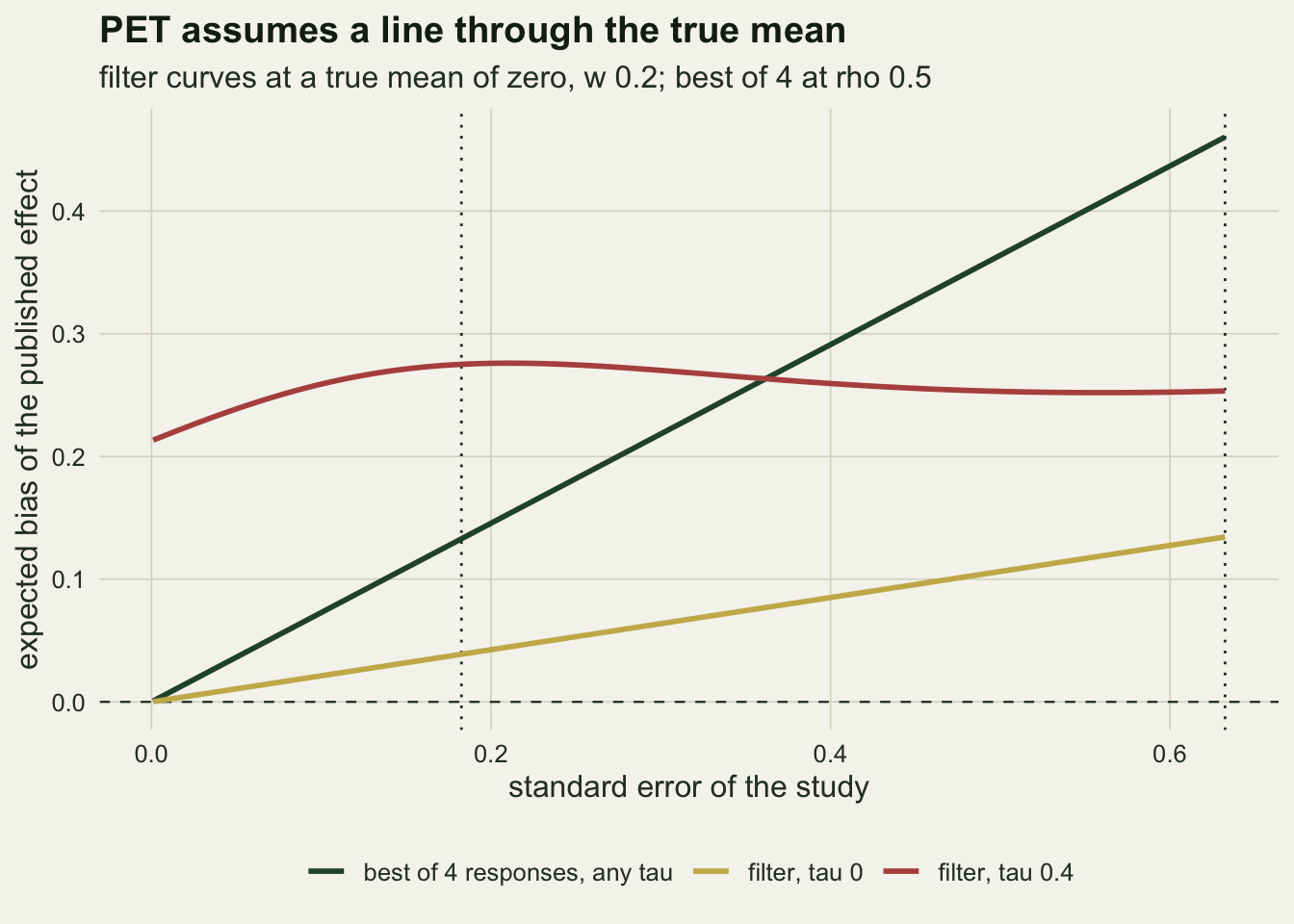
The filter under heterogeneity
The simulation grid crosses the number of studies (10, 30, 60), the true mean (0, 0.3), tau (0, 0.2, 0.4) and the publication probability of non-significant studies (0.2 and 1), with 2000 syntheses in each of the 36 cells. Every synthesis is scored by every estimator, so the estimators are compared on the same literatures. Bias and root mean squared error are taken over the syntheses in a cell; Egger’s rate is the share of those syntheses with a two-sided p below 0.10.
n_rep <- 2000
est_names <- c("re", "pet", "peese", "pp1", "pp2", "pp3", "petre", "tf")
run_cell <- function(gen, mu) {
  r <- t(replicate(n_rep, { d <- gen(); fit_all(d$y, d$se) }))
  err <- r[, est_names] - mu
  c(bias = colMeans(err), mcse = apply(err, 2, sd) / sqrt(n_rep),
    rmse = sqrt(colMeans(err^2)),
    cov_re = mean(r[, "re_lo"] < mu & r[, "re_hi"] > mu),
    cov_pet = mean(r[, "pet_lo"] < mu & r[, "pet_hi"] > mu),
    cov_pp = mean(r[, "pp_lo"] < mu & r[, "pp_hi"] > mu),
    wid_re = mean(r[, "re_hi"] - r[, "re_lo"]),
    wid_pet = mean(r[, "pet_hi"] - r[, "pet_lo"]),
    i2_med = median(r[, "i2"]), i2_80 = mean(r[, "i2"] > 0.8),
    egger = mean(r[, "egger"]), switch = mean(r[, "switch"]))
}
grid_a <- expand.grid(k = c(10, 30, 60), mu = c(0, 0.3), tau = c(0, 0.2, 0.4),
                      w = c(0.2, 1))
set.seed(2014)
res_a <- cbind(grid_a, do.call(rbind, lapply(seq_len(nrow(grid_a)), function(i)
  run_cell(function() draw_filter(grid_a$k[i], grid_a$mu[i], grid_a$tau[i],
                                  grid_a$w[i]), grid_a$mu[i]))))
ga <- function(col, k, mu, tau, w) {
  res_a[res_a$k == k & res_a$mu == mu & res_a$tau == tau & res_a$w == w, col]
}
egger_se <- function(p) sqrt(p * (1 - p) / n_rep)
filt <- res_a[res_a$w == 0.2, ]
n_re_wins <- sum(filt$rmse.re < filt$rmse.pp1)
n_pp_less_biased <- sum(abs(filt$bias.pp1) < abs(filt$bias.re))
bias_ratio <- filt$bias.re / abs(filt$bias.pp1)
ratio_mu0 <- range(bias_ratio[filt$mu == 0 & filt$tau > 0])
ratio_mu3 <- range(bias_ratio[filt$mu == 0.3])
pp_win_cells <- filt[filt$rmse.pp1 <= filt$rmse.re, c("k", "mu", "tau")]
stopifnot(all(pp_win_cells$k == 60 & pp_win_cells$mu == 0.3))
round(res_a[res_a$w == 0.2, c("k", "mu", "tau", "bias.re", "bias.pet", "bias.pp1",
                              "bias.tf", "rmse.re", "rmse.pp1", "i2_med", "i2_80",
                              "egger")], 3)
k mu tau bias.re bias.pet bias.pp1 bias.tf rmse.re rmse.pp1 i2_med i2_80
1 10 0.0 0.0 0.055 -0.002 -0.033 0.050 0.110 0.340 0.225 0.000
2 30 0.0 0.0 0.055 -0.002 -0.018 0.057 0.077 0.183 0.259 0.000
3 60 0.0 0.0 0.052 -0.001 -0.010 0.058 0.064 0.123 0.266 0.000
4 10 0.3 0.0 0.142 0.030 -0.018 0.120 0.163 0.318 0.019 0.000
5 30 0.3 0.0 0.142 0.031 0.035 0.117 0.149 0.177 0.057 0.000
6 60 0.3 0.0 0.141 0.036 0.080 0.114 0.145 0.137 0.058 0.000
7 10 0.0 0.2 0.131 0.144 0.085 0.125 0.180 0.442 0.556 0.015
8 30 0.0 0.2 0.131 0.132 0.089 0.136 0.150 0.228 0.576 0.000
9 60 0.0 0.2 0.130 0.131 0.099 0.140 0.139 0.172 0.575 0.000
10 10 0.3 0.2 0.193 0.065 0.013 0.161 0.215 0.382 0.324 0.004
11 30 0.3 0.2 0.191 0.082 0.076 0.153 0.199 0.216 0.374 0.000
12 60 0.3 0.2 0.191 0.088 0.123 0.147 0.196 0.181 0.383 0.000
13 10 0.0 0.4 0.277 0.262 0.182 0.246 0.327 0.640 0.764 0.356
14 30 0.0 0.4 0.272 0.294 0.222 0.244 0.290 0.361 0.775 0.320
15 60 0.0 0.4 0.271 0.292 0.235 0.242 0.280 0.300 0.780 0.302
16 10 0.3 0.4 0.294 0.168 0.094 0.242 0.326 0.529 0.636 0.141
17 30 0.3 0.4 0.286 0.174 0.143 0.219 0.297 0.301 0.683 0.062
18 60 0.3 0.4 0.286 0.176 0.194 0.201 0.292 0.264 0.688 0.019
egger
1 0.103
2 0.109
3 0.126
4 0.159
5 0.198
6 0.243
7 0.082
8 0.083
9 0.058
10 0.124
11 0.145
12 0.168
13 0.071
14 0.067
15 0.063
16 0.100
17 0.095
18 0.105pp_win_cells k mu tau
6 60 0.3 0.0
12 60 0.3 0.2
18 60 0.3 0.4Take thirty studies, a true mean of zero, tau 0.4 and a filter that publishes a fifth of the non-significant results. Random effects is biased by 0.272. PET is biased by 0.294, PEESE by 0.281 and the conditional PET-PEESE estimator by 0.222, each with a Monte Carlo standard error no larger than 0.008. The correction does not correct: PET is further from the truth than the uncorrected mean, and the conditional estimator removes 0.050 of it while its root mean squared error rises from 0.290 to 0.361. The closed form above said as much: PET is aiming at an intercept of 0.296. With sixty studies PET’s bias is 0.292, so more studies change nothing.
Egger’s test, which is what would have prompted the correction, flags 0.067 of those syntheses (Monte Carlo standard error 0.006), below its own nominal 0.10 on a literature that is heavily filtered. The funnel does not lean in the way the test looks for, because the filter shifts precise and imprecise studies alike. The multilevel form of PET behaves as the plain one: its bias in the same cell is 0.295, since modelling tau-squared changes the weights but not the shape of the curve being extrapolated.
Without heterogeneity the same filter is the case PET handles. At tau 0 and a true mean of zero, thirty studies, random effects is biased by 0.055 and PET by -0.002; at a true mean of 0.3 the figures are 0.142 and 0.031, and the conditional estimator reaches 0.035. At tau 0.4 and a true mean of 0.3 the conditional estimator is still biased by 0.143 against 0.286 for random effects. Trim-and-fill, the comparison the blog already has, is biased by 0.244 in the zero-mean, tau 0.4 cell, and its root mean squared error of 0.269 is lower than the conditional estimator’s, because it barely moves the estimate and so adds little variance.
Stanley (2017) found conventional meta-analysis much worse than PET-PEESE, with random effects at least twice as biased, and advised against using any method once I-squared exceeds 0.8. On bias this grid agrees in direction: the conditional estimator is less biased than random effects in 18 of the 18 filtered cells. The margin is not twofold where the failure above sits: with heterogeneity and a true mean of zero, random effects is between 1.16 and 1.54 times as biased as the conditional estimator (0.272 against 0.222 at thirty studies and tau 0.4), while at a true mean of 0.3 the ratio runs from 1.47 to 14.7. In that thirty-study, tau 0.4 cell the median I-squared is 0.775 and 0.320 of the syntheses are above 0.8, so part of the grid lies where Stanley would fit nothing. Stanley’s comparison is framed on bias and type I error. On root mean squared error, the measure this post leads with, random effects beats the conditional estimator in 15 of the 18 filtered cells, and the 3 cells where PET-PEESE wins all have sixty studies and a true mean of 0.3. The designs differ in the selection rule, the sample sizes and the effect metric, and this post does not try to settle which is closer to ecology.
long_a <- do.call(rbind, lapply(c("re", "pet", "pp1", "tf"), function(e) {
  sub_a <- res_a[res_a$w == 0.2, ]
  data.frame(k = paste(sub_a$k, "studies"), mu = paste("true mean", sub_a$mu),
             tau = sub_a$tau, bias = sub_a[[paste0("bias.", e)]], est = e)
}))
long_a$k <- factor(long_a$k, levels = c("10 studies", "30 studies", "60 studies"))
long_a$est <- factor(long_a$est, levels = c("re", "pet", "pp1", "tf"),
                     labels = c("random effects", "PET", "PET-PEESE", "trim-and-fill"))
est_cols <- c("random effects" = te_ink, "PET" = te_forest,
              "PET-PEESE" = te_rust, "trim-and-fill" = te_gold)
ggplot(long_a, aes(tau, bias, colour = est)) +
  geom_hline(yintercept = 0, linetype = "dashed", colour = te_body, linewidth = 0.4) +
  geom_line(linewidth = 0.8) +
  geom_point(size = 1.8) +
  facet_grid(mu ~ k) +
  scale_colour_manual(values = est_cols, name = NULL) +
  scale_x_continuous(breaks = c(0, 0.2, 0.4)) +
  labs(x = "tau (between-site standard deviation)", y = "bias",
       title = "Heterogeneity turns the filter into a bias PET cannot see",
       subtitle = "filter publishes every significant positive study and 1 in 5 of the rest") +
  theme_datasheet() +
  theme(legend.position = "bottom",
        strip.text = element_text(colour = te_ink))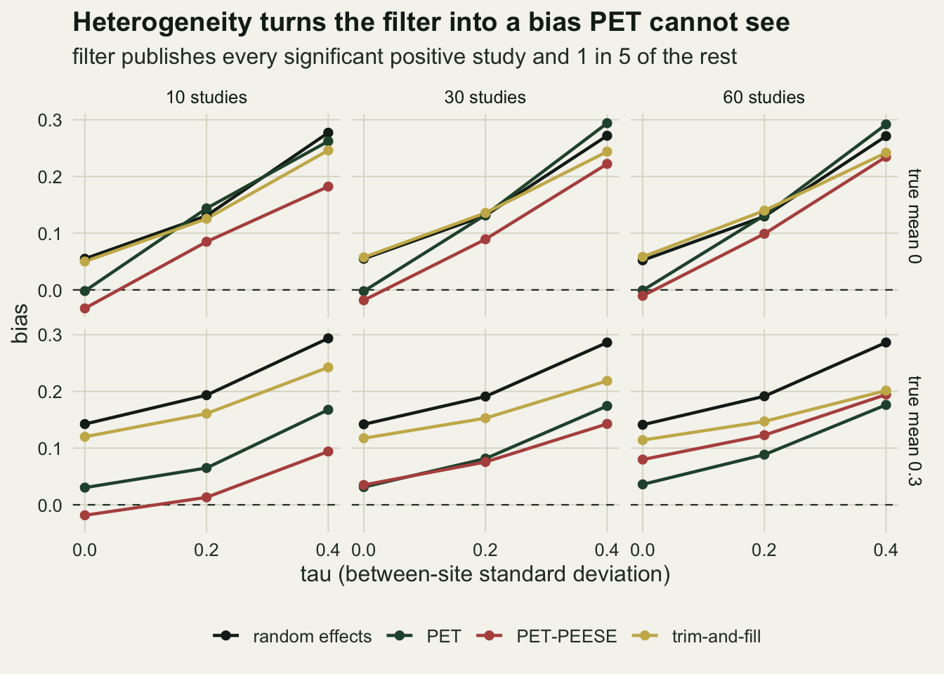
Correcting a literature that was never filtered
A correction is fitted because a funnel leans, and a funnel can lean for other reasons. With the publication probability set to one the literature is a fair sample, the random effects mean is unbiased, and the question is what the correction costs.
nosel <- res_a[res_a$w == 1, ]
nosel$ratio_pp1 <- nosel$rmse.pp1 / nosel$rmse.re
nosel$ratio_pp2 <- nosel$rmse.pp2 / nosel$rmse.re
nosel$ratio_pp3 <- nosel$rmse.pp3 / nosel$rmse.re
nosel$ratio_tf  <- nosel$rmse.tf / nosel$rmse.re
ratio_k10 <- ga("rmse.pp1", 10, 0.3, 0, 1) / ga("rmse.re", 10, 0.3, 0, 1)
ratio_lo <- min(nosel$ratio_pp1); ratio_hi <- max(nosel$ratio_pp1)
k60 <- nosel[nosel$k == 60, ]
gap_05 <- range(nosel$ratio_pp2 - nosel$ratio_pp1)
gap_neg <- nosel$ratio_pp2 - nosel$ratio_pp3   # effect of also switching on a negative intercept
i_neg <- which(nosel$mu == 0)[which.max(gap_neg[nosel$mu == 0])]
i_neg3 <- which(nosel$mu == 0.3)[which.max(abs(gap_neg[nosel$mu == 0.3]))]
ratio_any_min <- min(unlist(nosel[, c("ratio_pp1", "ratio_pp2", "ratio_pp3")]))
wid_ratio <- ga("wid_pet", 30, 0.3, 0, 1) / ga("wid_re", 30, 0.3, 0, 1)
pp1_bias_min <- min(nosel$bias.pp1)
round(nosel[, c("k", "mu", "tau", "rmse.re", "rmse.pp1", "rmse.pp2", "rmse.pp3",
                "ratio_pp1", "ratio_pp2", "ratio_pp3", "ratio_tf", "bias.pp1",
                "switch")], 3)
k mu tau rmse.re rmse.pp1 rmse.pp2 rmse.pp3 ratio_pp1 ratio_pp2 ratio_pp3
19 10 0.0 0.0 0.078 0.290 0.304 0.276 3.710 3.887 3.536
20 30 0.0 0.0 0.046 0.151 0.160 0.143 3.250 3.438 3.075
21 60 0.0 0.0 0.032 0.105 0.111 0.096 3.296 3.477 3.015
22 10 0.3 0.0 0.082 0.261 0.273 0.268 3.190 3.338 3.267
23 30 0.3 0.0 0.047 0.138 0.139 0.139 2.939 2.959 2.959
24 60 0.3 0.0 0.032 0.087 0.092 0.092 2.691 2.860 2.860
25 10 0.0 0.2 0.106 0.371 0.397 0.361 3.485 3.735 3.391
26 30 0.0 0.2 0.060 0.190 0.200 0.178 3.166 3.323 2.956
27 60 0.0 0.2 0.042 0.133 0.141 0.126 3.179 3.365 3.006
28 10 0.3 0.2 0.105 0.337 0.355 0.344 3.208 3.372 3.271
29 30 0.3 0.2 0.060 0.165 0.166 0.165 2.731 2.750 2.742
30 60 0.3 0.2 0.043 0.113 0.115 0.115 2.598 2.647 2.647
31 10 0.0 0.4 0.152 0.542 0.568 0.524 3.567 3.738 3.448
32 30 0.0 0.4 0.091 0.277 0.291 0.264 3.051 3.201 2.906
33 60 0.0 0.4 0.064 0.198 0.208 0.184 3.109 3.260 2.888
34 10 0.3 0.4 0.152 0.530 0.563 0.524 3.490 3.703 3.448
35 30 0.3 0.4 0.088 0.251 0.259 0.252 2.842 2.926 2.847
36 60 0.3 0.4 0.063 0.176 0.177 0.175 2.786 2.802 2.774
ratio_tf bias.pp1 switch
19 1.132 -0.024 0.092
20 1.244 -0.017 0.113
21 1.340 -0.014 0.097
22 1.090 -0.056 0.374
23 1.228 -0.037 0.658
24 1.305 -0.014 0.881
25 1.188 -0.038 0.111
26 1.347 -0.018 0.086
27 1.564 -0.016 0.093
28 1.181 -0.055 0.294
29 1.361 -0.042 0.532
30 1.483 -0.024 0.748
31 1.304 -0.063 0.083
32 1.558 -0.022 0.097
33 1.899 -0.025 0.090
34 1.342 -0.080 0.212
35 1.587 -0.061 0.343
36 1.911 -0.046 0.528With ten studies, a true mean of 0.3 and no heterogeneity, the conditional estimator has a root mean squared error of 0.261 against 0.082 for random effects, 3.2 times as large. Across the whole unfiltered grid the ratio runs from 2.60 to 3.71, and at sixty studies it is still between 2.60 and 3.30. The reason is extrapolation: the intercept is a prediction at a standard error of zero from studies whose standard errors start at 0.183, so it carries the uncertainty of a regression line read off far outside its data. PET’s interval is honest about this; at thirty studies and tau 0 its average width is 0.702 against 0.188 for random effects, 3.7 times as wide.
The conditional estimator is also biased downwards when nothing was filtered, by as much as 0.080, because the switch to PEESE depends on PET’s intercept being significant: the rule keeps PET when it came out low and replaces it when it came out high. The stricter one-sided 0.05 switch raises the ratio above Stanley’s rule by between 0.02 and 0.25. The unpublished two-sided 0.10 variant is the one-sided 0.05 test on the positive side plus a switch to PEESE when PET’s intercept is significantly negative, which pulls those estimates back towards zero. Against the one-sided 0.05 rule that extra switch lowers the ratio most at a true mean of zero, by 0.46 at 60 studies and tau 0 (3.48 against 3.01); at a true mean of 0.3 the largest change is 0.25, at 10 studies and tau 0.4. Under all three rules the ratio stays at or above 2.60.
nosel$tau_lab <- factor(paste("tau", nosel$tau))
nosel$mu_lab <- paste("true mean", nosel$mu)
ggplot(nosel, aes(k, ratio_pp1, colour = tau_lab)) +
  geom_hline(yintercept = 1, linetype = "dashed", colour = te_body, linewidth = 0.4) +
  geom_line(linewidth = 0.9) +
  geom_point(size = 2.2) +
  facet_wrap(~ mu_lab) +
  scale_colour_manual(values = c(te_forest, te_gold, te_rust), name = NULL) +
  scale_x_continuous(breaks = c(10, 30, 60)) +
  scale_y_continuous(limits = c(0, NA)) +
  labs(x = "number of studies", y = "RMSE of PET-PEESE / RMSE of random effects",
       title = "A correction with nothing to correct",
       subtitle = "every study published; one-sided 0.10 switching rule") +
  theme_datasheet() +
  theme(legend.position = "bottom",
        strip.text = element_text(colour = te_ink))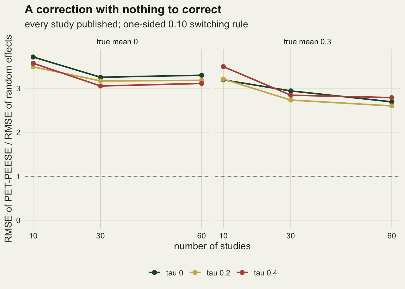
Selection within a study is the case PET was built for
The within-study grid holds thirty studies and a true mean of 0.3, reports the largest of four responses, and crosses tau (0, 0.2, 0.4) with the correlation among responses (0.2, 0.5, 0.8). Four more cells vary the number of studies at rho 0.5. PET’s unbiasedness is already known from the closed form; what the simulation adds is how the uncorrected bias compares with that arithmetic, what the correction costs in precision, and how often Egger’s test would have asked for it.
grid_b <- rbind(expand.grid(k = 30, tau = c(0, 0.2, 0.4), rho = c(0.2, 0.5, 0.8)),
                expand.grid(k = c(10, 60), tau = c(0, 0.4), rho = 0.5))
mu_b <- 0.3
set.seed(2017)
res_b <- cbind(grid_b, do.call(rbind, lapply(seq_len(nrow(grid_b)), function(i)
  run_cell(function() draw_within(grid_b$k[i], mu_b, grid_b$tau[i], m_resp,
                                  grid_b$rho[i]), mu_b))))
gb <- function(col, k, tau, rho) {
  res_b[res_b$k == k & res_b$tau == tau & res_b$rho == rho, col]
}
cf_rho <- sapply(c(0.2, 0.5, 0.8), function(r) e_max4 * sqrt(1 - r) * mean_se)
pet_b_max <- max(abs(res_b$bias.pet))
pet_b_mcse <- max(res_b$mcse.pet)
pet_b_z <- max(abs(res_b$bias.pet) / res_b$mcse.pet)
cf_share <- range(res_b$bias.re[res_b$k == 30 & res_b$tau == 0] / cf_rho)
round(res_b[, c("k", "tau", "rho", "bias.re", "bias.pet", "bias.pp1", "rmse.re",
                "rmse.pet", "cov_re", "cov_pet", "egger")], 3)
k tau rho bias.re bias.pet bias.pp1 rmse.re rmse.pet cov_re cov_pet egger
1 30 0.0 0.2 0.221 0.004 0.097 0.224 0.130 0.000 0.954 0.511
2 30 0.2 0.2 0.227 -0.004 0.041 0.233 0.186 0.010 0.958 0.300
3 30 0.4 0.2 0.242 0.005 0.000 0.256 0.289 0.162 0.966 0.140
4 30 0.0 0.5 0.176 0.004 0.060 0.180 0.149 0.013 0.955 0.317
5 30 0.2 0.5 0.180 -0.002 0.019 0.189 0.197 0.099 0.955 0.198
6 30 0.4 0.5 0.190 0.006 -0.015 0.209 0.305 0.399 0.954 0.107
7 30 0.0 0.8 0.112 0.001 0.018 0.120 0.165 0.336 0.947 0.183
8 30 0.2 0.8 0.114 -0.001 -0.009 0.128 0.211 0.500 0.959 0.127
9 30 0.4 0.8 0.121 0.005 -0.030 0.150 0.314 0.711 0.957 0.083
10 10 0.0 0.5 0.177 0.007 -0.004 0.191 0.284 0.410 0.952 0.164
11 60 0.0 0.5 0.175 -0.001 0.094 0.178 0.102 0.000 0.956 0.538
12 10 0.4 0.5 0.191 -0.018 -0.068 0.243 0.585 0.720 0.962 0.074
13 60 0.4 0.5 0.192 0.003 0.017 0.201 0.211 0.122 0.954 0.179At rho 0.5 and tau 0.4 the random effects mean is biased by 0.190 and PET by +0.006. Over all thirteen cells PET’s bias never exceeds 0.018 in absolute value, and no cell is more than 1.3 of its own Monte Carlo standard errors from zero. That is the closed form confirmed, not a separate result. The uncorrected bias follows its arithmetic too, at a fixed fraction below it: the unweighted closed form gives 0.263, 0.208 and 0.132 at rho 0.2, 0.5 and 0.8, and random effects at tau 0 comes out at 0.221, 0.176 and 0.112, between 0.84 and 0.85 of the unweighted value, because the weights favour precise studies, whose bias is smaller.
The bias of random effects is large enough to matter and its interval misses: at rho 0.5 its coverage of the true mean is 0.013 at tau 0 and 0.399 at tau 0.4, while PET’s interval covers 0.954. The price is precision. At tau 0.4 PET’s root mean squared error is 0.305 against 0.209 for the biased mean, so an analyst who cares about squared error rather than about bias would still prefer the uncorrected estimate in that cell.
What makes the repair mostly theoretical is detection. At rho 0.5, Egger’s test flags 0.317 of syntheses when tau is 0 and 0.107 when tau is 0.4 (Monte Carlo standard error 0.007); even at sixty studies and tau 0.4 it flags 0.179. Heterogeneity adds scatter at every standard error, the slope of a line through that scatter is poorly estimated, and a correction triggered by a significant slope is rarely triggered. The literature with the bias PET can remove is the literature in which the usual test does not ask for PET.
eg_df <- rbind(
  data.frame(tau = c(0, 0.2, 0.4), rate = sapply(c(0, 0.2, 0.4), function(tt)
    ga("egger", 30, 0, tt, 0.2)), arm = "filter, true mean 0"),
  data.frame(tau = c(0, 0.2, 0.4), rate = sapply(c(0, 0.2, 0.4), function(tt)
    ga("egger", 30, 0.3, tt, 0.2)), arm = "filter, true mean 0.3"),
  data.frame(tau = c(0, 0.2, 0.4), rate = sapply(c(0, 0.2, 0.4), function(tt)
    gb("egger", 30, tt, 0.5)), arm = "best of 4, rho 0.5"))
p_eg <- ggplot(eg_df, aes(tau, rate, colour = arm)) +
  geom_hline(yintercept = 0.10, linetype = "dashed", colour = te_body, linewidth = 0.4) +
  geom_line(linewidth = 0.9) + geom_point(size = 2) +
  scale_colour_manual(values = c("best of 4, rho 0.5" = te_forest,
                                 "filter, true mean 0" = te_gold,
                                 "filter, true mean 0.3" = te_rust), name = NULL) +
  scale_x_continuous(breaks = c(0, 0.2, 0.4)) +
  scale_y_continuous(limits = c(0, NA)) +
  labs(x = "tau", y = "share flagged by Egger's test", title = "Rarely asked for") +
  theme_datasheet() +
  theme(legend.position = "bottom", legend.direction = "vertical")
rb <- res_b[res_b$k == 30 & res_b$tau == 0.4, ]
bias_df <- rbind(
  data.frame(rho = rb$rho, bias = rb$bias.re, est = "random effects"),
  data.frame(rho = rb$rho, bias = rb$bias.pet, est = "PET"),
  data.frame(rho = c(0.2, 0.5, 0.8), bias = cf_rho, est = "closed form"))
p_bias <- ggplot(bias_df, aes(rho, bias, colour = est, linetype = est)) +
  geom_hline(yintercept = 0, linetype = "dashed", colour = te_body, linewidth = 0.4) +
  geom_line(linewidth = 0.9) + geom_point(size = 2) +
  scale_colour_manual(values = c("random effects" = te_ink, "PET" = te_forest,
                                 "closed form" = "grey45"), name = NULL) +
  scale_linetype_manual(values = c("random effects" = "solid", "PET" = "solid",
                                   "closed form" = "dotted"), name = NULL) +
  scale_x_continuous(breaks = c(0.2, 0.5, 0.8)) +
  labs(x = "correlation among responses", y = "bias", title = "Repaired by construction") +
  theme_datasheet() +
  theme(legend.position = "bottom", legend.direction = "vertical")
(p_eg | p_bias) + plot_annotation(theme = theme_datasheet())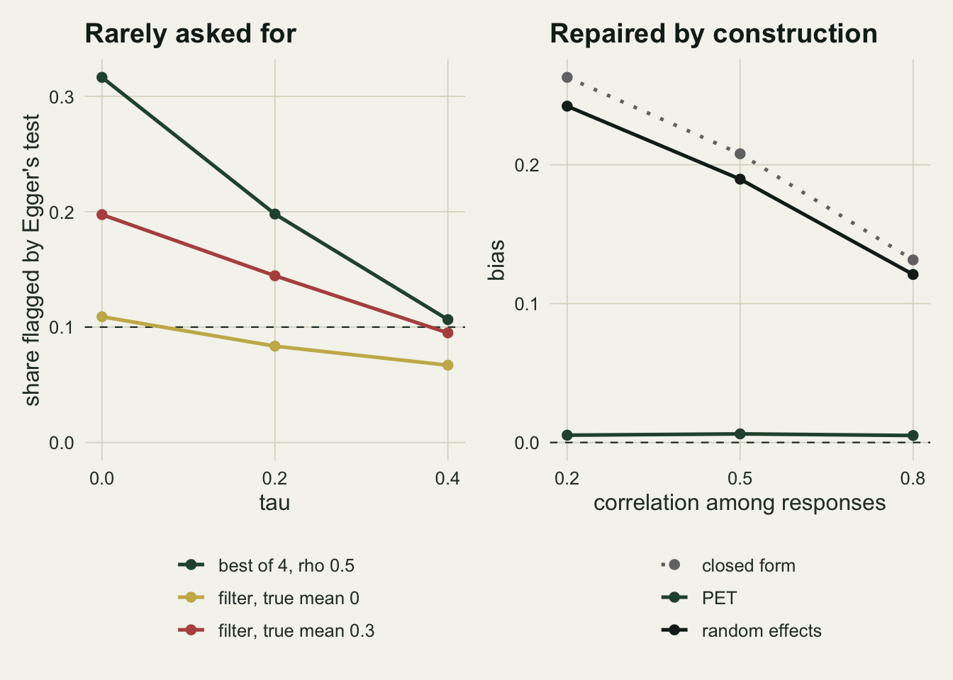
When the best response is chosen by its p value
The within-study result depends on every response having the same standard error, so that choosing the largest effect and choosing the smallest p value are the same act. Ecological responses rarely share a scale. Richness might be counted on a few quadrats and biomass weighed on many, and after standardisation their standard errors still differ through reliability and subsampling. An author choosing by p value then picks responses with small standard errors more often when the study’s true effect is positive, and the reported standard error starts to carry information about the true effect.
sd_scale <- 0.4     # log scale spread of the standard error among a study's responses
draw_pick_p <- function(k, mu, tau, m, rho) {
  s0 <- sqrt(2 / sample(n_min:n_max, k, TRUE))
  s_mat <- s0 * exp(matrix(rnorm(k * m, 0, sd_scale), k, m))
  z <- sqrt(rho) * rnorm(k) + sqrt(1 - rho) * matrix(rnorm(k * m), k, m)
  y_mat <- rnorm(k, mu, tau) + s_mat * z
  pick <- max.col(y_mat / s_mat, ties.method = "first")
  idx <- cbind(seq_len(k), pick)
  list(y = y_mat[idx], se = s_mat[idx])
}
grid_p <- expand.grid(mu = c(0, 0.3), tau = c(0, 0.4))
set.seed(2019)
res_p <- cbind(grid_p, do.call(rbind, lapply(seq_len(nrow(grid_p)), function(i)
  run_cell(function() draw_pick_p(30, grid_p$mu[i], grid_p$tau[i], m_resp, rho_mid),
           grid_p$mu[i]))))
gp <- function(col, mu, tau) res_p[res_p$mu == mu & res_p$tau == tau, col]
round(res_p[, c("mu", "tau", "bias.re", "bias.pet", "bias.pp1", "bias.petre",
                "mcse.pet", "egger")], 3)
mu tau bias.re bias.pet bias.pp1 bias.petre mcse.pet egger
1 0.0 0.0 0.144 0.000 0.001 0.000 0.002 0.626
2 0.3 0.0 0.079 -0.077 0.018 -0.077 0.002 0.811
3 0.0 0.4 0.206 0.416 0.305 0.330 0.004 0.287
4 0.3 0.4 0.165 0.242 0.197 0.209 0.004 0.137With the standard error of each response spread by a factor whose log has standard deviation 0.4, thirty studies, rho 0.5 and the smallest p value reported, PET is still unbiased at a true mean of zero and no heterogeneity: its bias is 0.000 in absolute value (Monte Carlo standard error 0.002), because with no true effect the choice by p value ignores the standard error and the reported effect is the standard error times a selected standard normal. As soon as the true effects are positive the choice favours precise responses. At a true mean of 0.3 and tau 0, PET overcorrects to -0.077, against 0.079 for random effects, already 51 Monte Carlo standard errors from zero where PET’s bias in the equal-scale grid never exceeded 0.018 in absolute value. At tau 0.4 it breaks outright: PET’s bias is 0.416 at a true mean of zero, against 0.206 for random effects, and 0.242 against 0.165 at 0.3. A response with a smaller standard error turns the same true effect into a larger z. Once the true effect is positive, a precise response wins the choice with a modest sampling error and an imprecise one only with a large error, so the expected bias is no longer proportional to the standard error and PET’s straight line misses the true mean. With heterogeneity, studies with larger true effects report their most precise responses more often, the smallest standard errors go with the largest effects, and the intercept is pulled up. This is the between-study problem again, arriving through a within-study choice.
What to report
Report the uncorrected random effects estimate and tau next to any PET-PEESE result, and treat a large tau as a reason not to trust the correction rather than as a detail. At tau 0.4 with a filter and thirty studies, the conditional estimator was biased by 0.222 at a true mean of zero, and doubling to sixty studies left PET at 0.292.
Do not use a non-significant Egger test as evidence that no correction is needed, or a significant one as the gate for fitting it. Under the filter at tau 0.4, Egger’s test flagged 0.067 of syntheses; under best-of-four reporting at the same tau it flagged 0.107.
Say which switching rule was used and give PET’s interval, not only the point estimate. On an unfiltered literature of thirty studies PET’s interval was 3.7 times as wide as that of random effects, and a corrected estimate quoted without it looks far more informative than it is.
Say how the effect sizes were chosen from each study. If a protocol took the first reported response, or all responses, the within-study bias is absent; if it took the one the authors emphasised, it is present, and whether a regression correction can remove it depends on whether the responses share a scale. With several responses per study, the three-level model in the dependent effect sizes post is the place to put them, and it removes the choice.
Honest limits
The sampling variances are known and depend only on sample size. Real standardised mean differences carry an estimated variance that depends on the effect itself, which creates funnel asymmetry with no selection. None of that is simulated, so the no-selection costs above are a best case.
The filter is a single hard step at the two-sided 0.05 boundary with one publication probability. Real selection is graded and may depend on the size of an effect as well as on its p value. The mechanism shown in the closed form, a filter that still acts on precise studies once their true effects differ, does not depend on the shape of the step, but the numbers do.
The standard errors come from per arm sample sizes spread evenly between 5 and 60. The cost of PET is mostly the cost of extrapolating to a standard error of zero, so a literature with a few very large studies would pay less and one in which every study is small would pay more. Stanley (2017) makes the same point about samples that are all small.
The multilevel PET here is a random effects meta-regression with a moment estimate of tau-squared and one effect per study. The model Nakagawa and colleagues describe is fitted by restricted maximum likelihood with study and observation levels and, often, a variance rather than a standard error as moderator. With one effect per study the levels collapse, and the result above suggests that the estimator of tau-squared is not what drives the failure, but a REML fit was not run.
Trim-and-fill (Duval and Tweedie 2000, the L0 estimator) trims around a fixed effect centre as the funnel post does; unlike that post, the filled set is pooled by random effects here. Other implementations trim with the random effects centre and will give somewhat different numbers.
The within-study case has four equicorrelated responses with a common correlation and, in its main form, a common standard error. Real responses are correlated unevenly and are chosen by rules that mix effect size, p value and ecological interest. The p value variant shows that a modest spread of standard errors is enough to break PET under heterogeneity, and the spread chosen, 0.4 on the log scale, is a design constant rather than an estimate from any literature.
References
Stanley TD, Doucouliagos H 2014 Research Synthesis Methods 5(1):60-78 (10.1002/jrsm.1095)
Stanley TD 2017 Social Psychological and Personality Science 8(5):581-591 (10.1177/1948550617693062)
Carter EC, Schonbrodt FD, Gervais WM, Hilgard J 2019 Advances in Methods and Practices in Psychological Science 2(2):115-144 (10.1177/2515245919847196)
Nakagawa S, Lagisz M, Jennions MD, Koricheva J, Noble DWA, Parker TH, Sanchez-Tojar A, Yang Y, O’Dea RE 2022 Methods in Ecology and Evolution 13(1):4-21 (10.1111/2041-210X.13724)
Egger M, Davey Smith G, Schneider M, Minder C 1997 BMJ 315(7109):629-634 (10.1136/bmj.315.7109.629)
Duval S, Tweedie R 2000 Biometrics 56(2):455-463 (10.1111/j.0006-341X.2000.00455.x)
DerSimonian R, Laird N 1986 Controlled Clinical Trials 7(3):177-188 (10.1016/0197-2456(86)90046-2)