library(ggplot2)
library(patchwork)

te_paper  <- "#f5f4ee"
te_ink    <- "#16241d"
te_body   <- "#2c3a31"
te_forest <- "#275139"
te_rust   <- "#b5534e"
te_gold   <- "#c9b458"
te_line   <- "#dad9ca"

theme_datasheet <- function() {
  theme_minimal(base_size = 12) +
    theme(plot.background  = element_rect(fill = te_paper, colour = NA),
          panel.background = element_rect(fill = te_paper, colour = NA),
          panel.grid.major = element_line(colour = te_line, linewidth = 0.3),
          panel.grid.minor = element_blank(),
          text             = element_text(colour = te_body),
          plot.title       = element_text(colour = te_ink, face = "bold"),
          plot.subtitle    = element_text(colour = te_body),
          axis.text        = element_text(colour = te_body))
}Inclusion criteria move the pooled effect
R
meta-analysis
publication bias
research synthesis
simulation
ecology tutorial
An English-only screening rule shifts a pooled effect as the funnel plot and Egger test stay quiet. Measuring in R what inclusion rules do to a meta-analysis.
A synthesis of livestock exclusion experiments collects every study that compares plant species richness inside and outside a fence, and turns each one into a standardised mean difference. The studies come from two grassland regions. In the first, everything is published in English. In the second, a large share of the field work appears in national journals, written in the national language, and those papers are hard to find with the usual search strings and harder still to read. The protocol, written before the search, says English language papers only. Nobody thinks of that line as a modelling decision.
It is one. The random effects model that pools the studies estimates the mean true effect of whatever studies are fed to it, and the screening rules decide what gets fed. If a rule removes studies at random with respect to their effects, it costs precision and nothing else. If the rule is correlated with a moderator, and language is correlated with region almost by definition, then the rule changes the study mix and the pooled mean moves with it. Konno and colleagues raise the same concern from real ecological syntheses, where leaving out the non-English studies could change the overall mean effect considerably.
The site already has the tools that are normally run to check whether a pooled effect can be trusted. Random-effects meta-analysis in R builds the DerSimonian and Laird estimator used below. Heterogeneity in meta-analysis computes I-squared and shows that it is a relative measure that rises with study size. Checking for publication bias draws the funnel plot and runs Egger’s regression, which look for small studies with systematically different results, and selection models for publication bias write a filter into the likelihood whose probability of keeping a study depends on its p value. All of that machinery is built around missingness that depends on the result or on the precision of a study. A language rule depends on neither. This post measures what that rule does to the pooled effect, to I-squared and to Egger’s test, and then asks how far the answer moves across all sixteen combinations of four ordinary inclusion rules.
Two hundred studies and a stated target
The generating model is written down before anything is estimated, and every constant in it was fixed before the first run. Each region contributes one hundred studies. The true effect of a study is its regional mean, plus a small decline with publication year, plus independent study level variation. Sample size per arm is drawn on a log scale and has nothing to do with region or effect. Each study carries three attributes that a protocol might screen on: whether it is in a national language journal, whether it is grey literature such as a thesis or agency report, and its year.
k_reg    <- 100                          # studies per region
mu_reg   <- c(A = 0.60, B = 0.20)        # regional mean true effect (Hedges g)
tau_w    <- 0.15                         # study level SD inside a region
p_local  <- c(A = 0.00, B = 0.40)        # share in national language journals
p_grey   <- c(A = 0.15, B = 0.35)        # share of grey literature
yr_lo    <- 1990; yr_hi <- 2023          # publication years, uniform
yr_mid   <- (yr_lo + yr_hi) / 2
yr_slope <- -0.006                       # change in true effect per year
n_lo     <- 8; n_hi <- 80                # per arm sample size, log uniform
n_min    <- 20                           # minimum sample size rule
yr_min   <- 2000                         # date range rule
z_crit   <- qnorm(0.975)

make_studies <- function(p_loc = p_local, mu = mu_reg, slope = yr_slope,
                         tau = tau_w, p_gr = p_grey) {
  region <- rep(c("A", "B"), each = k_reg)
  k_all  <- length(region)
  year   <- sample(yr_lo:yr_hi, k_all, replace = TRUE)
  n_arm  <- round(exp(runif(k_all, log(n_lo), log(n_hi))))
  theta  <- mu[region] + slope * (year - yr_mid) + rnorm(k_all, 0, tau)
  v_samp <- 2 / n_arm                    # large sample variance of g, equal arms
  data.frame(region, year, n_arm, theta, v_samp,
             g_obs = rnorm(k_all, theta, sqrt(v_samp)),
             local = runif(k_all) < p_loc[region],
             grey  = runif(k_all) < p_gr[region])
}
The target has to be defined before a filter can be said to depart from it. Here it is the mean true effect over every eligible study that was carried out, in both regions and in every language. The regions contribute equally and the year term is centred on the middle of the publication window, so that mean is 0.40 by construction. A review could legitimately want a different target, such as the effect in region A alone, but then region A is its question, and a protocol that says so would screen on region, not on language.
The estimator is DerSimonian and Laird’s: a fixed effect mean, Cochran’s Q around it, a moment estimate of the between study variance truncated at zero, and a second weighted mean with weights one over the sampling variance plus that estimate. I-squared is Higgins and Thompson’s, Q minus its degrees of freedom over Q. Egger’s test regresses each standardised effect, the estimate over its standard error, on its precision, one over the standard error, and tests the intercept against zero with a t statistic on k minus two degrees of freedom. All three are written out by hand.
dl_fit <- function(g, v) {
  k_s  <- length(g); w <- 1 / v
  m_fe <- sum(w * g) / sum(w)
  q_st <- sum(w * (g - m_fe)^2)
  tau2 <- max(0, (q_st - (k_s - 1)) / (sum(w) - sum(w^2) / sum(w)))
  w_re <- 1 / (v + tau2)
  c(mu = sum(w_re * g) / sum(w_re), se = sqrt(1 / sum(w_re)), tau2 = tau2,
    i2 = max(0, (q_st - (k_s - 1)) / q_st), k = k_s)
}

egger_p <- function(g, v) {
  s_e <- sqrt(v); z_std <- g / s_e; prec <- 1 / s_e
  k_s <- length(g); x_bar <- mean(prec)
  b1  <- sum((prec - x_bar) * (z_std - mean(z_std))) / sum((prec - x_bar)^2)
  b0  <- mean(z_std) - b1 * x_bar
  s2  <- sum((z_std - b0 - b1 * prec)^2) / (k_s - 2)
  se0 <- sqrt(s2 * (1 / k_s + x_bar^2 / sum((prec - x_bar)^2)))
  2 * pt(-abs(b0 / se0), df = k_s - 2)
}
The English-only rule on one synthesis
One simulated literature first, analysed twice: once with every study and once after the language rule.
set.seed(8190)
lit <- make_studies()
keep_en <- !lit$local
fit_all <- dl_fit(lit$g_obs, lit$v_samp)
fit_en  <- dl_fit(lit$g_obs[keep_en], lit$v_samp[keep_en])
eg_all  <- egger_p(lit$g_obs, lit$v_samp)
eg_en   <- egger_p(lit$g_obs[keep_en], lit$v_samp[keep_en])
ci_all  <- fit_all[["mu"]] + c(-1, 1) * z_crit * fit_all[["se"]]
ci_en   <- fit_en[["mu"]]  + c(-1, 1) * z_crit * fit_en[["se"]]
n_drop  <- sum(!keep_en)
check_lm <- summary(lm(I(g_obs / sqrt(v_samp)) ~ I(1 / sqrt(v_samp)),
                       data = lit))$coefficients[1, 4]
round(rbind(all = fit_all, english = fit_en), 3)
mu se tau2 i2 k
all 0.39 0.030 0.089 0.562 200
english 0.45 0.033 0.085 0.552 155The rule removes 45 of the 200 studies, all from region B. With every study the pooled effect is 0.390, 95 per cent interval 0.332 to 0.448, which contains the target of 0.40. After the rule it is 0.450, interval 0.385 to 0.514. I-squared goes from 0.562 to 0.552, and the Egger p value from 0.254 to 0.680. The hand coded Egger test agrees with lm() on the full set to 5.6e-16, so the formula is the ordinary regression and not an approximation of it.
lit$status <- ifelse(lit$local, "removed by English-only rule",
                     ifelse(lit$region == "A", "kept, region A", "kept, region B"))
se_seq <- seq(0, max(sqrt(lit$v_samp)) * 1.05, length.out = 50)
funnel_df <- data.frame(se = c(se_seq, rev(se_seq)),
                        g  = c(fit_all[["mu"]] - z_crit * se_seq,
                               rev(fit_all[["mu"]] + z_crit * se_seq)))
line_df <- data.frame(g = c(fit_all[["mu"]], fit_en[["mu"]]),
                      fit = c("all studies", "English only"))
ggplot(lit, aes(g_obs, sqrt(v_samp))) +
  geom_polygon(data = funnel_df, aes(g, se), fill = NA, colour = te_line,
               linetype = "dashed", linewidth = 0.4) +
  geom_vline(data = line_df, aes(xintercept = g, linetype = fit),
             colour = te_ink, linewidth = 0.6) +
  geom_point(aes(colour = status, shape = status), size = 2.2, alpha = 0.85) +
  scale_y_reverse() +
  scale_colour_manual(values = c("kept, region A" = te_forest,
                                 "kept, region B" = te_gold,
                                 "removed by English-only rule" = te_rust)) +
  scale_shape_manual(values = c(16, 16, 4)) +
  scale_linetype_manual(values = c("all studies" = "solid", "English only" = "dotted"),
                        breaks = c("all studies", "English only")) +
  labs(x = "Observed effect (Hedges g)", y = "Standard error",
       colour = NULL, shape = NULL, linetype = NULL) +
  theme_datasheet() +
  theme(legend.position = "bottom", legend.box = "vertical")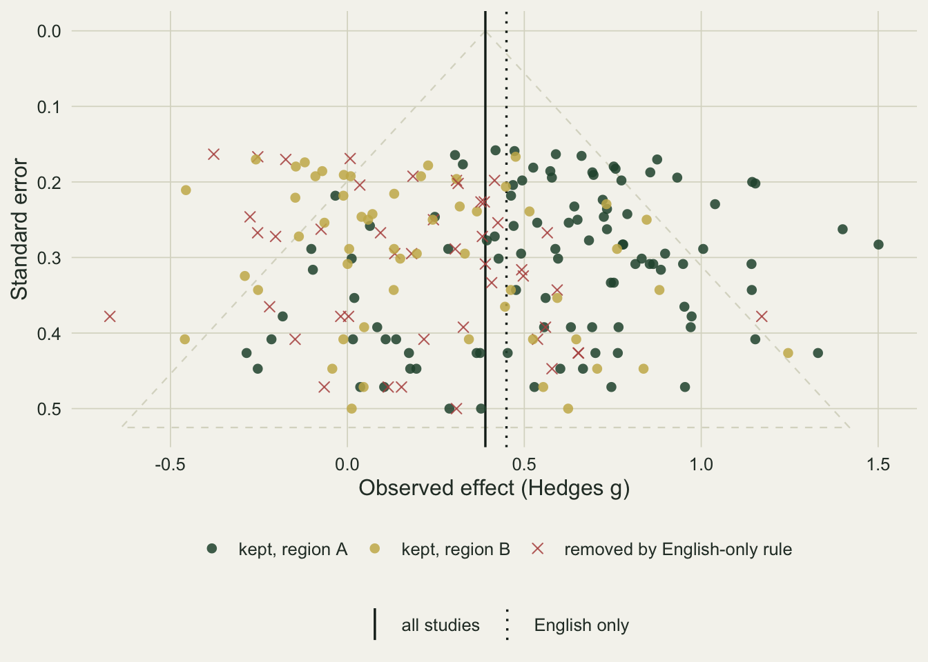
Two thousand syntheses
One dataset shows the mechanism; a rate needs replication. The same two analyses are repeated on two thousand independent literatures, with the four screening rules and their sixteen combinations evaluated inside the same loop so that later sections reuse it.
n_rep  <- 2000
rule_grid <- as.matrix(expand.grid(language = 0:1, size = 0:1,
                                   peer = 0:1, date = 0:1))
keep_rules <- function(d, code) {
  keep <- rep(TRUE, nrow(d))
  if (code[1] == 1) keep <- keep & !d$local
  if (code[2] == 1) keep <- keep & d$n_arm >= n_min
  if (code[3] == 1) keep <- keep & !d$grey
  if (code[4] == 1) keep <- keep & d$year >= yr_min
  keep
}
run_one <- function(...) {
  d <- make_studies(...)
  en <- !d$local; b_all <- d$region == "B"; b_en <- b_all & en
  f_all <- dl_fit(d$g_obs, d$v_samp); f_en <- dl_fit(d$g_obs[en], d$v_samp[en])
  multi <- apply(rule_grid, 1, function(cd) {
    kk <- keep_rules(d, cd); dl_fit(d$g_obs[kk], d$v_samp[kk])[c("mu", "se")]
  })
  c(mu_all = f_all[["mu"]], se_all = f_all[["se"]], tau2_all = f_all[["tau2"]],
    i2_all = f_all[["i2"]], mu_en = f_en[["mu"]], se_en = f_en[["se"]],
    tau2_en = f_en[["tau2"]], i2_en = f_en[["i2"]], k_en = f_en[["k"]],
    eg_all = egger_p(d$g_obs, d$v_samp), eg_en = egger_p(d$g_obs[en], d$v_samp[en]),
    true_en = mean(d$theta[en]),
    muB_all = dl_fit(d$g_obs[b_all], d$v_samp[b_all])[["mu"]],
    muB_en  = dl_fit(d$g_obs[b_en], d$v_samp[b_en])[["mu"]],
    mv_range = diff(range(multi["mu", ])),
    mv_width = median(2 * z_crit * multi["se", ]),
    mv_min = min(multi["mu", ]), mv_max = max(multi["mu", ]))
}
set.seed(8191)
mc <- as.data.frame(t(vapply(seq_len(n_rep), function(i) run_one(), numeric(18))))

target  <- mean(mu_reg)
mse     <- function(x) sd(x) / sqrt(length(x))
rate_se <- function(p) sqrt(p * (1 - p) / n_rep)
bias_all <- mean(mc$mu_all) - target; bias_en <- mean(mc$mu_en) - target
cov_all <- mean(abs(mc$mu_all - target) < z_crit * mc$se_all)
cov_en  <- mean(abs(mc$mu_en - target) < z_crit * mc$se_en)
rej_all <- mean(mc$eg_all < 0.05); rej_en <- mean(mc$eg_en < 0.05)
shift_in_se <- mean((mc$mu_en - target) / mc$se_en)
i2_drop <- round(mean(mc$i2_all), 3) - round(mean(mc$i2_en), 3)   # agrees with the printed means
i2_sd   <- sd(mc$i2_all)
own_gap <- mean(mc$mu_en - mc$true_en)
Across 2000 literatures the pooled effect with every study averages 0.400 (Monte Carlo standard error 0.0005) against the target of 0.40. After the English-only rule it averages 0.450 (standard error 0.0006), a shift of 0.050, which is on average 1.7 times the standard error that the filtered analysis reports for itself. The planned shift for this design was larger; the measured one follows from plain arithmetic, because removing forty per cent of region B leaves region B with 37.5 per cent of the studies, and a mix of that share at 0.20 and the rest at 0.60 has a mean of 0.450.
The interval from the full analysis contains the target in 98.2 per cent of literatures (Monte Carlo standard error 0.3), well above nominal because the model treats the fixed fifty to fifty split of regions as if it were random between study variance. The interval from the English-only analysis contains the target in 61.2 per cent (standard error 1.1).
Nothing is wrong with the estimator. The filtered pooled effect differs from the mean true effect of the studies it actually used by 0.0002 on average. It answers its own question correctly; the rule changed the question.
The checks do not notice. Egger’s test rejects at the five per cent level in 4.3 per cent of full literatures and in 4.8 per cent of filtered ones (standard errors 0.5 and 0.5): both are within two Monte Carlo standard errors of the nominal five per cent, which is what a test whose null is true should give. The language of a study is unrelated to its standard error, so the removed studies are spread evenly from the top to the bottom of the funnel, and a funnel that loses a symmetric slice stays symmetric. I-squared falls by 0.013 on average, from 0.505 to 0.492. The plan for this post expected a large fall that would make the filtered synthesis look cleaner. The fall is in the direction that reads as an improvement, but it is well under half of the literature to literature standard deviation of I-squared itself, 0.049, so no reader of a single synthesis could see it. Neither check improves in any useful sense; both simply stay where they were.
Why I-squared barely moves
The size of that fall is mechanical. Between study variance in this design has three parts: the study level variance inside a region, the year term, and the spread of the two regional means around the overall mean. That last part is the share of region B times the share of region A times the squared difference of the regional means. A product of two shares that sum to one is flat near a half, so removing forty per cent of one region barely changes it. To see where I-squared starts to fall, the removal share is swept from none of region B to all of it.
drop_share <- seq(0, 1, by = 0.1)
n_rep_sw   <- 400
var_year   <- ((yr_hi - yr_lo + 1)^2 - 1) / 12
exp_tau2 <- function(f) {
  share_b <- (1 - f) / (2 - f)
  share_b * (1 - share_b) * diff(mu_reg)^2 + tau_w^2 + yr_slope^2 * var_year
}
set.seed(8192)
sweep_tab <- do.call(rbind, lapply(drop_share, function(f) {
  p_f <- c(A = 0, B = f)
  sims <- vapply(seq_len(n_rep_sw), function(i) {
    d <- make_studies(p_loc = p_f)
    dl_fit(d$g_obs[!d$local], d$v_samp[!d$local])[c("mu", "tau2", "i2")]
  }, numeric(3))
  data.frame(f = f, mu = mean(sims["mu", ]), mu_se = mse(sims["mu", ]),
             tau2 = mean(sims["tau2", ]), i2 = mean(sims["i2", ]),
             i2_se = mse(sims["i2", ]), tau2_exp = exp_tau2(f),
             mu_exp = (mu_reg[["A"]] + (1 - f) * mu_reg[["B"]]) / (2 - f))
}))
tau2_gap <- max(abs(sweep_tab$tau2 - sweep_tab$tau2_exp))
i2_at <- function(f) sweep_tab$i2[abs(sweep_tab$f - f) < 1e-9]
The expected between study variance with every study is 0.0660, and the regional part of it is 0.0400. With forty per cent of region B removed the regional part is 0.0375, so the total only falls to 0.0635. The simulated DerSimonian and Laird means sit within 0.0010 of that curve at every removal share. I-squared follows, because it is tau-squared over tau-squared plus a typical sampling variance, and the rule does not change study sizes, so the typical sampling variance stays where it was: 0.501 with no studies removed, 0.490 at forty per cent, 0.416 at eighty per cent, and 0.267 only when region B has gone entirely. The pooled effect, in contrast, moves steadily from the first study removed, because its expected value is a weighted mean that is linear in region B’s share of the kept studies, while the regional part of the variance is a product of shares that is flat near a half.
sw_base <- ggplot(sweep_tab, aes(x = 100 * f)) +
  labs(x = "B removed (%)") + theme_datasheet() +
  theme(plot.title = element_text(size = 12))
p_mu <- sw_base +
  geom_hline(yintercept = target, colour = te_rust, linetype = "dashed") +
  geom_line(aes(y = mu_exp), colour = te_line, linewidth = 1.2) +
  geom_errorbar(aes(ymin = mu - 2 * mu_se, ymax = mu + 2 * mu_se),
                width = 0, colour = te_forest) +
  geom_point(aes(y = mu), colour = te_forest, size = 2) +
  labs(y = "Pooled effect", title = "Pooled effect")
p_tau <- sw_base +
  geom_line(aes(y = tau2_exp), colour = te_line, linewidth = 1.2) +
  geom_point(aes(y = tau2), colour = te_gold, size = 2) +
  labs(y = "Tau-squared", title = "Tau-squared")
p_i2 <- sw_base +
  geom_errorbar(aes(ymin = i2 - 2 * i2_se, ymax = i2 + 2 * i2_se),
                width = 0, colour = te_ink) +
  geom_point(aes(y = i2), colour = te_ink, size = 2) +
  labs(y = "I-squared", title = "I-squared")
p_mu + p_tau + p_i2 + plot_annotation(theme = theme_datasheet())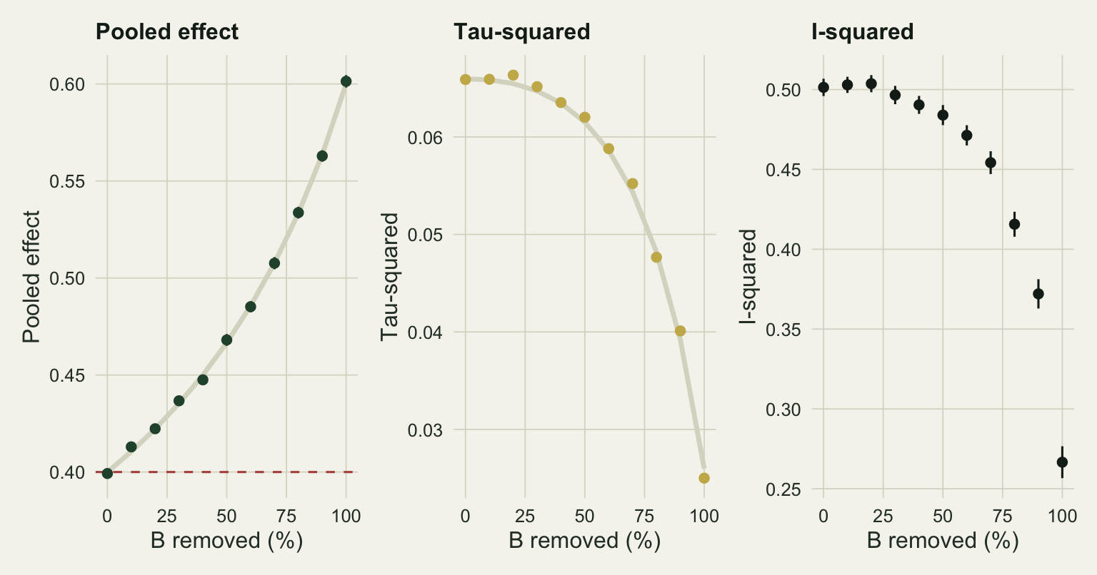
A region moderator sees what the funnel cannot
The filter moves the pooled effect only because it is correlated with region. Inside region B it removes studies at random with respect to their effects, so an analysis that estimates region B on its own should not move.
muB_all_m <- mean(mc$muB_all); muB_en_m <- mean(mc$muB_en)
muB_diff_se <- mse(mc$muB_en - mc$muB_all)
Averaged over the same 2000 literatures, the region B estimate is 0.200 from all of its studies and 0.201 from the English ones, a difference of 0.0007 with a Monte Carlo standard error of 0.0006, against a regional true mean of 0.20. The subgroup estimate is less precise after the rule, because it rests on fewer studies, but it is not shifted. This is the practical defence: when a screening rule is known to track a moderator, report the moderator, and let a reader combine the regional estimates with whatever weights their question needs. The post on meta-regression with moderators fits the same idea with a continuous moderator; region would enter that weighted regression as a zero or one column.
Sixteen protocols, one literature
Language is one rule among several that every protocol sets. Here are four, each defensible on its own: English only; at least 20 samples per arm; peer reviewed papers only; published in 2000 or later. In this design the size rule is unrelated to the effect, the peer review rule removes more of region B than of region A, and the date rule removes older studies, whose true effects are larger. Crossing the four gives sixteen protocols, the multiverse in the sense of Steegen and colleagues, all applied to the literature from the first section.
rule_label <- function(code) {
  nm <- c("English", paste("n >=", n_min), "peer reviewed",
          paste(">=", yr_min))[code == 1]
  if (length(nm) == 0) "no rules" else paste(nm, collapse = " + ")
}
mv_one <- do.call(rbind, lapply(seq_len(nrow(rule_grid)), function(j) {
  kk <- keep_rules(lit, rule_grid[j, ])
  fj <- dl_fit(lit$g_obs[kk], lit$v_samp[kk])
  data.frame(protocol = rule_label(rule_grid[j, ]), mu = fj[["mu"]],
             lo = fj[["mu"]] - z_crit * fj[["se"]], hi = fj[["mu"]] + z_crit * fj[["se"]],
             k = fj[["k"]], n_rules = sum(rule_grid[j, ]))
}))
mv_range_one <- diff(range(mv_one$mu))
mv_width_one <- median(mv_one$hi - mv_one$lo)
k_span <- range(mv_one$k)
lo_prot <- mv_one$protocol[which.min(mv_one$mu)]
hi_prot <- mv_one$protocol[which.max(mv_one$mu)]
mv_one
protocol mu lo hi
1 no rules 0.3899547 0.3318823 0.4480270
2 English 0.4495884 0.3846834 0.5144934
3 n >= 20 0.3908809 0.3189396 0.4628222
4 English + n >= 20 0.4594113 0.3800028 0.5388198
5 peer reviewed 0.4206939 0.3541727 0.4872151
6 English + peer reviewed 0.4758057 0.4067125 0.5448988
7 n >= 20 + peer reviewed 0.4248180 0.3432281 0.5064078
8 English + n >= 20 + peer reviewed 0.4926748 0.4109588 0.5743907
9 >= 2000 0.3500308 0.2818300 0.4182315
10 English + >= 2000 0.3970907 0.3219951 0.4721864
11 n >= 20 + >= 2000 0.3560761 0.2691998 0.4429523
12 English + n >= 20 + >= 2000 0.4084531 0.3143941 0.5025122
13 peer reviewed + >= 2000 0.3873910 0.3081072 0.4666749
14 English + peer reviewed + >= 2000 0.4335215 0.3517867 0.5152564
15 n >= 20 + peer reviewed + >= 2000 0.4051979 0.3066892 0.5037066
16 English + n >= 20 + peer reviewed + >= 2000 0.4646566 0.3674268 0.5618864
k n_rules
1 200 0
2 155 1
3 119 1
4 94 2
5 143 1
6 119 2
7 87 2
8 73 3
9 141 1
10 112 2
11 80 2
12 65 3
13 100 2
14 84 3
15 60 3
16 51 4The sixteen pooled effects run from 0.350 under “>= 2000” to 0.493 under “English + n >= 20 + peer reviewed”, a range of 0.143, on between 51 and 200 studies. The median width of their 95 per cent intervals is 0.159.
mv_one$protocol <- factor(mv_one$protocol, levels = mv_one$protocol[order(mv_one$mu)])
ggplot(mv_one, aes(mu, protocol)) +
  geom_vline(xintercept = target, colour = te_rust, linetype = "dashed") +
  geom_segment(aes(x = lo, xend = hi, yend = protocol), colour = te_line, linewidth = 1.6) +
  geom_point(aes(colour = factor(n_rules), shape = factor(n_rules)), size = 2.6) +
  scale_colour_manual(values = c("0" = te_ink, "1" = te_forest, "2" = te_gold,
                                 "3" = te_rust, "4" = te_ink),
                      name = "Rules applied") +
  scale_shape_manual(values = c("0" = 16, "1" = 16, "2" = 16, "3" = 16, "4" = 17),
                     name = "Rules applied") +
  labs(x = "Pooled effect (Hedges g)", y = NULL) +
  theme_datasheet() +
  theme(legend.position = "bottom")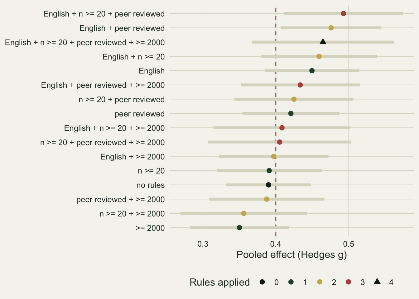
Whether a range is wide or narrow needs a comparison that is fair to the interval. The range of sixteen estimates is not a sampling quantity: the protocols share most of their studies, so it is smaller than it would be for independent literatures, and it would not be zero even if no rule tracked any moderator, because every subset drops a different random handful of studies. The fair yardstick is therefore a null multiverse that keeps everything that sets the size of that subsetting noise and removes only the link between rules and effects. It has the same regional means, the same total between study variance (the year term is folded into the study level variance, so there is no trend for the date rule to catch), the same overall shares of national language and grey literature, but those shares are equal in the two regions, so no rule tracks region. The comparison is made against the median interval width across the sixteen protocols, which is wider than the full data interval and so favours the interval.
set.seed(8193)
tau_null   <- sqrt(tau_w^2 + yr_slope^2 * var_year)       # same total variance
p_loc_null <- c(A = mean(p_local), B = mean(p_local))  # same overall shares,
p_gr_null  <- c(A = mean(p_grey), B = mean(p_grey))    # equal in both regions
mc_null <- as.data.frame(t(vapply(seq_len(n_rep), function(i)
  run_one(p_loc = p_loc_null, slope = 0, tau = tau_null, p_gr = p_gr_null),
  numeric(18))))
ratio_des  <- mc$mv_range / mc$mv_width
ratio_null <- mc_null$mv_range / mc_null$mv_width
over_des  <- mean(ratio_des > 1); over_null <- mean(ratio_null > 1)
miss_des  <- mean(mc$mv_min > target | mc$mv_max < target)
over_full <- mean(mc$mv_range > 2 * z_crit * mc$se_all)
null_mult <- mean(mc$mv_range) / mean(mc_null$mv_range)
tau2_des  <- mean(mc$tau2_all); tau2_null <- mean(mc_null$tau2_all)
In the design, the range of the sixteen estimates averages 0.123 against a median interval width of 0.138, and it exceeds that width in 28.4 per cent of literatures (Monte Carlo standard error 1.0). Measured against the narrower interval of the analysis with no rules, the range is wider in 71.6 per cent. In the null multiverse the range averages 0.062 against a width of 0.140, and exceeds it in 0.0 per cent.
So the planned claim, that the rules give a range wider than the reported interval, depends on which interval is chosen. Against the fair yardstick it holds in a minority of literatures; the typical range is a little narrower than a typical interval. What does hold is the comparison with the null. Its median interval width, 0.140, matches the design’s 0.138, and its mean tau-squared with every study, 0.0664, matches the design’s 0.0666, so the two carry comparable subsetting noise; against that, the designed range is 2.0 times the null range. The extra spread the rules add, 0.061 on average, is a little under half a typical interval width, and no single protocol’s interval accounts for any of it. The target sits outside the range of all sixteen estimates in 10.4 per cent of designed literatures, so the full set of protocols brackets the target more often than the English-only interval covers it.
ratio_df <- rbind(data.frame(ratio = ratio_des,  scenario = "rules track moderators"),
                  data.frame(ratio = ratio_null, scenario = "null: rules track no moderator"))
ggplot(ratio_df, aes(ratio, fill = scenario)) +
  geom_histogram(binwidth = 0.05, boundary = 0, position = "identity", alpha = 0.7,
                 colour = NA) +
  geom_vline(xintercept = 1, colour = te_ink, linetype = "dashed") +
  scale_fill_manual(values = c("rules track moderators" = te_rust,
                               "null: rules track no moderator" = te_forest),
                    name = NULL) +
  labs(x = "Range of sixteen estimates / median interval width",
       y = "Literatures") +
  theme_datasheet() +
  theme(legend.position = "bottom")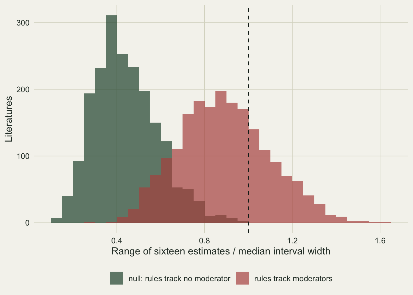
What to report
State the target in the protocol, in words, before the search: the mean effect across which studies, from which regions, over which years. A rule that cannot be defended as part of that definition is a convenience, and it should be reported as one.
For every rule that removes studies, report how many it removed and a comparison of those studies with the kept ones on the moderators the review records. A language rule that removes a fifth of the studies, all from one region, is a result, and a reader cannot reconstruct it from the flow diagram alone.
Do not cite a symmetric funnel or a non-significant Egger test as evidence that the included set is representative. Both answer a question about small studies. Neither can see a filter that is independent of study size, and I-squared can drift down slightly when a filter narrows the mix, which reads as the opposite of a warning.
Where a rule tracks a moderator, report the moderator estimates, as in the subgroup section above. Where several rules are in play, run the sixteen, or however many, protocols and report the range next to the interval of the chosen one, together with the protocol that gave each end.
Honest limits
The regions, their shares and their effects were chosen to make the mechanism visible. Real language filters are messier: non-English studies are not confined to one region, they may differ in design and sample size, and if they are smaller on average the language rule would also tilt the funnel, which would make Egger’s test react to a filter it would then misread as publication bias. The clean separation here, where nothing about a study’s size depends on its language, is the reason the checks stay silent, and it is a best case for the checks’ blindness rather than a typical one.
The target is a mixture mean, and a mixture mean is only as meaningful as the mixture. With regional effects of 0.60 and 0.20, a pooled value of 0.40 describes no region, and the honest summary of this literature is two numbers. The post uses the pooled mean because that is what most syntheses report, not because it is the right quantity here.
Nothing here involves publication bias proper. The missingness never depends on a result. Real literatures carry both kinds at once, and a screening rule can interact with a publication filter, for example when grey literature holds the non-significant results. That interaction is not measured.
The sampling variance of each effect is the large sample value, two over the per arm sample size, which ignores the small term that depends on the effect itself. With the exact variance of Hedges g a weak link between effect and standard error appears, the artefact that the post on publication bias mentions, and Egger’s rejection rates could drift away from nominal; that version was not run.
DerSimonian and Laird’s estimator was used throughout and REML was not run. REML would give somewhat different between study variances, most of all for the smaller protocols, and so different weights and intervals; the shift in the pooled effect, though, is driven by the study mix, which no choice of tau-squared estimator changes.
References
DerSimonian R, Laird N 1986 Controlled Clinical Trials 7(3):177-188 (10.1016/0197-2456(86)90046-2)
Egger M, Davey Smith G, Schneider M, Minder C 1997 BMJ 315(7109):629-634 (10.1136/bmj.315.7109.629)
Higgins JPT, Thompson SG 2002 Statistics in Medicine 21(11):1539-1558 (10.1002/sim.1186)
Konno K, Akasaka M, Koshida C, Katayama N, Osada N, Spake R, Amano T 2020 Ecology and Evolution 10(13):6373-6384 (10.1002/ece3.6368)
Steegen S, Tuerlinckx F, Gelman A, Vanpaemel W 2016 Perspectives on Psychological Science 11(5):702-712 (10.1177/1745691616658637)