library(ggplot2)
library(patchwork)
library(nlme)

te_paper  <- "#f5f4ee"
te_ink    <- "#16241d"
te_body   <- "#2c3a31"
te_forest <- "#275139"
te_rust   <- "#b5534e"
te_gold   <- "#c9b458"
te_line   <- "#dad9ca"

theme_datasheet <- function() {
  theme_minimal(base_size = 12) +
    theme(plot.background  = element_rect(fill = te_paper, colour = NA),
          panel.background = element_rect(fill = te_paper, colour = NA),
          panel.grid.major = element_line(colour = te_line, linewidth = 0.3),
          panel.grid.minor = element_blank(),
          text             = element_text(colour = te_body),
          plot.title       = element_text(colour = te_ink, face = "bold"),
          plot.subtitle    = element_text(colour = te_body),
          axis.text        = element_text(colour = te_body),
          strip.text       = element_text(colour = te_ink))
}Omitted random slopes and false positives
R
mixed models
nlme
type I error
simulation
ecology tutorial
A random intercept model that leaves out a real random slope finds a mean effect that is not there. Measuring in R why the slope variance test cannot warn you.
Ten grassland sites along a regional rainfall gradient, ten quadrats in each, and in every quadrat a soil moisture reading and a clipped biomass sample. The question is whether biomass rises with soil moisture within a site, on average across sites. Soil moisture varies from quadrat to quadrat, so the covariate lives inside the site, and the obvious model is a linear mixed model with a random intercept for site and a fixed slope for moisture.
The sites do not all respond the same way. On a deep loam the extra water turns into grass; on a thin soil over rock the wettest quadrats are the waterlogged ones and grow less. So each site has its own slope, and the population question is about the mean of those slopes. A model with a random intercept only forces a common slope on all ten sites, and it then treats all one hundred quadrats as independent evidence about that slope.
This site has already shown what that costs on one dataset. The post on random slopes in mixed models fits both models to twelve sites and finds the standard error of the fixed slope nearly doubling once the site slopes are allowed to vary, which is the point Schielzeth and Forstmeier 2009 made for behavioural ecology. That post measures no error rate. The post on random effects with too few levels does measure a conditional type I error, but its covariate is constant within a stream and the state it conditions on is a singular random intercept; no slope is omitted there. The two pseudoreplication posts, pseudoreplication and false positives and GLMMs for nested counts, count false positives when the random intercept itself is left out.
What is measured here is the omitted slope. The headline, that an intercept-only model rejects a true zero mean slope far too often when site slopes vary, is known: Schielzeth and Forstmeier 2009 and Barr and colleagues 2013 both show it, and this post demonstrates it rather than discovering it. The number this post adds is a conditional one. The usual defence against the problem is to test whether the slope variance is zero and to add the random slope only if that test says so. The question is how often that test fires in exactly the datasets where leaving the slope out produced a false positive.
One false positive, taken apart
Every design constant below was fixed before any simulation was run: ten quadrats per site, moisture drawn uniformly between minus one and one within each site (so its site means are zero in expectation and differ only by sampling), a site intercept standard deviation of one, a site slope standard deviation of 0.3, a residual standard deviation of 0.5 and a mean slope of zero. Both models are fitted by maximum likelihood with nlme::lme, so that the likelihood ratio test between them is legitimate and the fixed effect tests come from the same fits.
n_obs      <- 10      # quadrats per site
sd_int     <- 1       # site intercept standard deviation
sd_res     <- 0.5     # residual standard deviation
sd_slope0  <- 0.3     # site slope standard deviation, main design
j_set      <- c(6, 10, 20, 40)
alpha_lev  <- 0.05    # every test
alpha_sel  <- 0.2     # selection level used by Matuschek et al. 2017
ctl <- lmeControl(returnObject = TRUE, msMaxIter = 200, maxIter = 200)

make_sites <- function(J, sd_slope, mean_slope = 0) {
  site     <- factor(rep(seq_len(J), each = n_obs))
  slope_j  <- mean_slope + rnorm(J, 0, sd_slope)
  moisture <- runif(J * n_obs, -1, 1)
  biomass  <- rnorm(J, 0, sd_int)[site] + slope_j[site] * moisture +
              rnorm(J * n_obs, 0, sd_res)
  list(dat = data.frame(biomass, moisture, site), slope_j = slope_j)
}

# boundary mixture for adding a slope variance and its covariance (Stram and Lee)
p_mix <- function(lr) 0.5 * pchisq(lr, 1, lower.tail = FALSE) +
                      0.5 * pchisq(lr, 2, lower.tail = FALSE)
crit_mix <- uniroot(function(q) p_mix(q) - alpha_lev, c(0.1, 20))$root

fit_pair <- function(dat) {
  n_warn <- 0
  quiet <- function(expr) withCallingHandlers(expr, warning = function(w) {
    n_warn <<- n_warn + 1; invokeRestart("muffleWarning") })
  m_ri <- quiet(lme(biomass ~ moisture, random = ~ 1 | site, data = dat,
                    method = "ML", control = ctl))
  m_rs <- tryCatch(quiet(lme(biomass ~ moisture, random = ~ moisture | site,
                             data = dat, method = "ML", control = ctl)),
                   error = function(e) NULL)
  list(ri = m_ri, rs = m_rs, n_warn = n_warn)
}

# within-site test of slope heterogeneity: lm(site * x) against lm(site + x)
f_slopes <- function(dat) {
  xc <- dat$moisture - ave(dat$moisture, dat$site)
  yc <- dat$biomass - ave(dat$biomass, dat$site)
  sxx <- tapply(xc^2, dat$site, sum); sxy <- tapply(xc * yc, dat$site, sum)
  syy <- tapply(yc^2, dat$site, sum)
  J <- nlevels(dat$site); N <- nrow(dat)
  rss_full <- sum(syy - sxy^2 / sxx)
  rss_red  <- sum(syy) - sum(sxy)^2 / sum(sxx)
  f_stat <- ((rss_red - rss_full) / (J - 1)) / (rss_full / (N - 2 * J))
  c(p_f = pf(f_stat, J - 1, N - 2 * J, lower.tail = FALSE),
    p_site = t.test(sxy / sxx)$p.value)   # two-stage test on site slopes
}
The first draw with ten sites in which the intercept-only model declares a moisture effect is the worked example. Picking a false positive on purpose is the point of the section, and the choice rule is fixed: the first one in a seeded sequence.
set.seed(3170)
i_try <- 0
repeat {
  i_try <- i_try + 1
  ex <- make_sites(10, sd_slope0)
  ex_fit <- fit_pair(ex$dat)
  if (summary(ex_fit$ri)$tTable["moisture", 5] < alpha_lev) break
}
tt_ri <- summary(ex_fit$ri)$tTable["moisture", ]
tt_rs <- summary(ex_fit$rs)$tTable["moisture", ]
ex_lr <- as.numeric(2 * (logLik(ex_fit$rs) - logLik(ex_fit$ri)))
ex_plr <- p_mix(ex_lr)
ex_true_mean <- mean(ex$slope_j)
ex_se_ratio <- tt_rs[2] / tt_ri[2]
ex_f <- f_slopes(ex$dat)
ref_f <- anova(lm(biomass ~ site + moisture, data = ex$dat),
               lm(biomass ~ site * moisture, data = ex$dat))[2, 6]
f_gap <- abs(ex_f[["p_f"]] - ref_f)
It took 14 draws to get one. The intercept-only model estimates the mean slope at 0.172 with a standard error of 0.086 on 89 degrees of freedom, p = 0.048. The model with a random slope returns 0.143 with a standard error of 0.146, 1.71 times larger, and p = 0.329. The two point estimates are close; the standard errors are not. The ten true site slopes in this draw average -0.012, so there is nothing to find even among these particular sites. The estimate is noise from ten small within-site regressions with slopes that really differ, and the intercept-only standard error, which counts quadrats rather than sites, is too small to recognise it as noise.
The check that is meant to catch this gives a likelihood ratio statistic of 10.16 and a boundary mixture p value of 0.004. The within-site F test for different slopes gives p = 2.8e-04 (its closed form matches anova() on the two linear models to 5.9e-18). In this dataset both checks would have prompted the random slope, and the false positive would have been avoided. Whether that is typical of the false positives, or just of this one, is the question the rest of the post answers.
ex_lines <- do.call(rbind, lapply(split(ex$dat, ex$dat$site), function(s) {
  cf <- coef(lm(biomass ~ moisture, data = s))
  data.frame(site = s$site[1], moisture = c(-1, 1), biomass = cf[1] + cf[2] * c(-1, 1))
}))
pop <- rbind(
  data.frame(model = "random intercept only", moisture = c(-1, 1),
             biomass = fixef(ex_fit$ri)[1] + fixef(ex_fit$ri)[2] * c(-1, 1)),
  data.frame(model = "random intercept and slope", moisture = c(-1, 1),
             biomass = fixef(ex_fit$rs)[1] + fixef(ex_fit$rs)[2] * c(-1, 1)))
pop$model <- factor(pop$model, levels = c("random intercept only", "random intercept and slope"))
fan_one <- function(fit, tt, label) {
  xs <- seq(-1, 1, length.out = 41); q <- qt(1 - alpha_lev / 2, tt[3])
  data.frame(model = label, moisture = xs,
             lo = fixef(fit)[1] + pmin((tt[1] - q * tt[2]) * xs, (tt[1] + q * tt[2]) * xs),
             hi = fixef(fit)[1] + pmax((tt[1] - q * tt[2]) * xs, (tt[1] + q * tt[2]) * xs))
}
fans <- rbind(fan_one(ex_fit$ri, tt_ri, "random intercept only"),
              fan_one(ex_fit$rs, tt_rs, "random intercept and slope"))
fans$model <- factor(fans$model, levels = levels(pop$model))
ggplot(ex$dat, aes(moisture, biomass)) +
  geom_ribbon(data = fans, aes(x = moisture, ymin = lo, ymax = hi, fill = model),
              inherit.aes = FALSE, alpha = 0.3) +
  geom_point(colour = te_body, alpha = 0.35, size = 1.2) +
  geom_line(data = ex_lines, aes(group = site), colour = te_forest,
            linewidth = 0.5, alpha = 0.7) +
  geom_line(data = pop, aes(colour = model, linetype = model), linewidth = 1.4) +
  scale_colour_manual(values = c(te_rust, te_gold), name = NULL) +
  scale_fill_manual(values = c(te_rust, te_gold), name = NULL) +
  scale_linetype_manual(values = c("solid", "dashed"), name = NULL) +
  labs(x = "soil moisture (same range in every site)", y = "biomass (standardised units)",
       title = "Same slope, very different uncertainty",
       subtitle = "thin lines: each site's own fit; bands: 95 per cent interval for the mean slope") +
  theme_datasheet() + theme(legend.position = "bottom")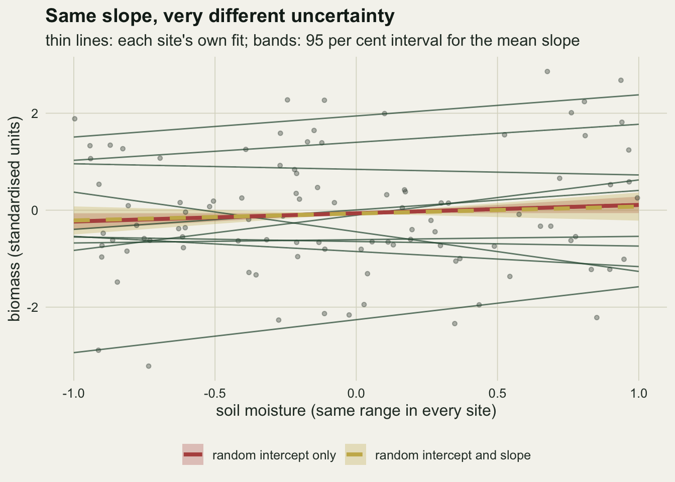
How often the intercept-only model is wrong
One dataset is an anecdote. The rate comes from repeating the whole thing, with both fits and both checks on every dataset. Each call below fits two mixed models, so the replicate count is the expensive constant, and it was set before any rate was inspected.
analyse_one <- function(J, sd_slope, mean_slope = 0) {
  s <- make_sites(J, sd_slope, mean_slope)
  ff <- fit_pair(s$dat)
  tt_ri <- summary(ff$ri)$tTable["moisture", ]
  if (is.null(ff$rs)) {
    t_rs <- NA; df_rs <- NA; lr <- NA
  } else {
    tt_rs <- summary(ff$rs)$tTable["moisture", ]
    t_rs <- tt_rs[[4]]; df_rs <- tt_rs[[3]]
    lr <- max(0, as.numeric(2 * (logLik(ff$rs) - logLik(ff$ri))))
  }
  c(t_ri = tt_ri[[4]], df_ri = tt_ri[[3]], t_rs = t_rs, df_rs = df_rs, lr = lr,
    f_slopes(s$dat), var_b = var(s$slope_j), mean_b = mean(s$slope_j),
    n_warn = ff$n_warn, J = J, sd_slope = sd_slope, mean_slope = mean_slope)
}

sim_cell <- function(n_rep, J, sd_slope, mean_slope = 0) {
  out <- as.data.frame(t(vapply(seq_len(n_rep), function(i)
    analyse_one(J, sd_slope, mean_slope), numeric(13))))
  out$rej_ri   <- 2 * pt(-abs(out$t_ri), out$df_ri) < alpha_lev
  out$rej_rs   <- 2 * pt(-abs(out$t_rs), out$df_rs) < alpha_lev
  out$rej_rs_j <- 2 * pt(-abs(out$t_rs), J - 1) < alpha_lev
  out$rej_site <- out$p_site < alpha_lev
  out$lrt      <- p_mix(out$lr) < alpha_lev
  out$f_fire   <- out$p_f < alpha_lev
  out$keep_sl  <- !is.na(out$lr) & p_mix(out$lr) < alpha_sel
  out$keep_chi <- !is.na(out$lr) & pchisq(out$lr, 2, lower.tail = FALSE) < alpha_sel
  out$rej_sel  <- ifelse(out$keep_sl, out$rej_rs, out$rej_ri)
  out
}

n_main <- 500     # per number of sites, slope SD 0.3
n_grid <- 250     # per cell of the slope SD grid (ten sites)
set.seed(41207)
t_start <- proc.time()[["elapsed"]]
main <- do.call(rbind, lapply(j_set, function(J) sim_cell(n_main, J, sd_slope0)))
set.seed(41208)
grid_cells <- expand.grid(J = 10, sd_slope = c(0, 0.15))
side <- do.call(rbind, lapply(seq_len(nrow(grid_cells)), function(k)
  sim_cell(n_grid, grid_cells$J[k], grid_cells$sd_slope[k])))
sim_secs <- proc.time()[["elapsed"]] - t_start
n_fail <- sum(is.na(c(main$lr, side$lr)))
share_warn <- mean(c(main$n_warn, side$n_warn) > 0)
rate_tab <- do.call(rbind, lapply(j_set, function(J) {
m <- main[main$J == J, ]
data.frame(J = J, model = c("random intercept only", "random intercept and slope"),
rate = c(mean(m$rej_ri), mean(m$rej_rs, na.rm = TRUE)))
}))
rate_tab$model <- factor(rate_tab$model, levels = c("random intercept only", "random intercept and slope"))
rate_tab$mcse <- sqrt(rate_tab$rate * (1 - rate_tab$rate) / n_main)
r_at <- function(J, k) rate_tab$rate[rate_tab$J == J & as.integer(rate_tab$model) == k]
mcse_nom <- sqrt(alpha_lev * (1 - alpha_lev) / n_main)
ri_range <- range(rate_tab$rate[as.integer(rate_tab$model) == 1])
pooled10 <- rbind(side, main[main$J == 10, ])
sd_tab <- do.call(rbind, lapply(c(0, 0.15, sd_slope0), function(s) {
m <- pooled10[pooled10$sd_slope == s, ]
data.frame(sd_slope = s, n = nrow(m),
ri = mean(m$rej_ri), rs = mean(m$rej_rs, na.rm = TRUE))
}))
sd_at <- function(s, col) sd_tab[sd_tab$sd_slope == s, col]
keep_share <- vapply(j_set, function(J) mean(main$keep_sl[main$J == J]), 0)
keep_chi_share <- vapply(j_set, function(J) mean(main$keep_chi[main$J == J]), 0)The simulation ran 2500 datasets in 75 seconds when this page was built. The random slope fit failed outright in 0 of them; 23.4 per cent produced at least one convergence warning, and those fits are kept as returned, as the software hands them over.
With a site slope standard deviation of 0.3 and a true mean slope of zero, the intercept-only model rejects at 17.2 per cent with six sites, 19.4 per cent with ten, 14.6 per cent with twenty and 14.4 per cent with forty. The Monte Carlo standard error near those values is about 1.6 percentage points. More sites do not repair it. The reason is in the standard error: the variance of the mean site slope is the slope variance divided by the number of sites, and the intercept-only standard error shrinks with the number of quadrats instead, so both fall at the same rate as sites are added and their ratio stays put.
The model with the random slope rejects at 9.8, 9.2, 7.2 and 5.0 per cent over the same four designs, against a Monte Carlo standard error of 1.0 points at the nominal rate. That is better, and at six sites it is still not five per cent; the degrees of freedom are part of the reason, and a later section comes back to them.
The damage grows with the slope variance. With ten sites the intercept-only model rejects 3.2 per cent of the time when the sites share one slope, 6.4 per cent at a slope standard deviation of 0.15 and 19.4 per cent at 0.3. The two grid cells carry 250 datasets each, so their Monte Carlo standard error is larger: 1.4 points at five per cent. The random slope model rejects at 3.2, 4.8 and 9.2 per cent over the same three values.
p_j <- ggplot(rate_tab, aes(J, rate, colour = model)) +
  geom_hline(yintercept = alpha_lev, colour = te_body, linetype = "dashed", linewidth = 0.5) +
  geom_errorbar(aes(ymin = rate - 2 * mcse, ymax = rate + 2 * mcse), width = 0.04, linewidth = 0.4) +
  geom_line(linewidth = 0.9) + geom_point(size = 2.2) +
  scale_x_log10(breaks = j_set) +
  scale_colour_manual(values = c(te_rust, te_forest), name = NULL) +
  scale_y_continuous(limits = c(0, NA)) +
  guides(colour = guide_legend(nrow = 2)) +
  labs(x = "sites (10 quadrats each)", y = "rejection rate under the null",
       title = "More sites do not help", subtitle = "bars: two Monte Carlo SE") +
  theme_datasheet() + theme(legend.position = "bottom")

sd_long <- rbind(data.frame(sd_tab[, c("sd_slope", "n")], model = "random intercept only", rate = sd_tab$ri),
                 data.frame(sd_tab[, c("sd_slope", "n")], model = "random intercept and slope", rate = sd_tab$rs))
sd_long$model <- factor(sd_long$model, levels = levels(rate_tab$model))
sd_long$mcse <- sqrt(sd_long$rate * (1 - sd_long$rate) / sd_long$n)
p_sd <- ggplot(sd_long, aes(sd_slope, rate, colour = model)) +
  geom_hline(yintercept = alpha_lev, colour = te_body, linetype = "dashed", linewidth = 0.5) +
  geom_errorbar(aes(ymin = rate - 2 * mcse, ymax = rate + 2 * mcse), width = 0.008, linewidth = 0.4) +
  geom_line(linewidth = 0.9) + geom_point(size = 2.2) +
  scale_colour_manual(values = c(te_rust, te_forest), guide = "none") +
  scale_x_continuous(breaks = c(0, 0.15, 0.3)) +
  scale_y_continuous(limits = c(0, NA)) +
  labs(x = "site slope standard deviation", y = NULL,
       title = "The slope variance drives it", subtitle = "ten sites, zero mean slope throughout") +
  theme_datasheet() + theme(legend.position = "bottom")

p_j + p_sd + plot_annotation(theme = theme_datasheet())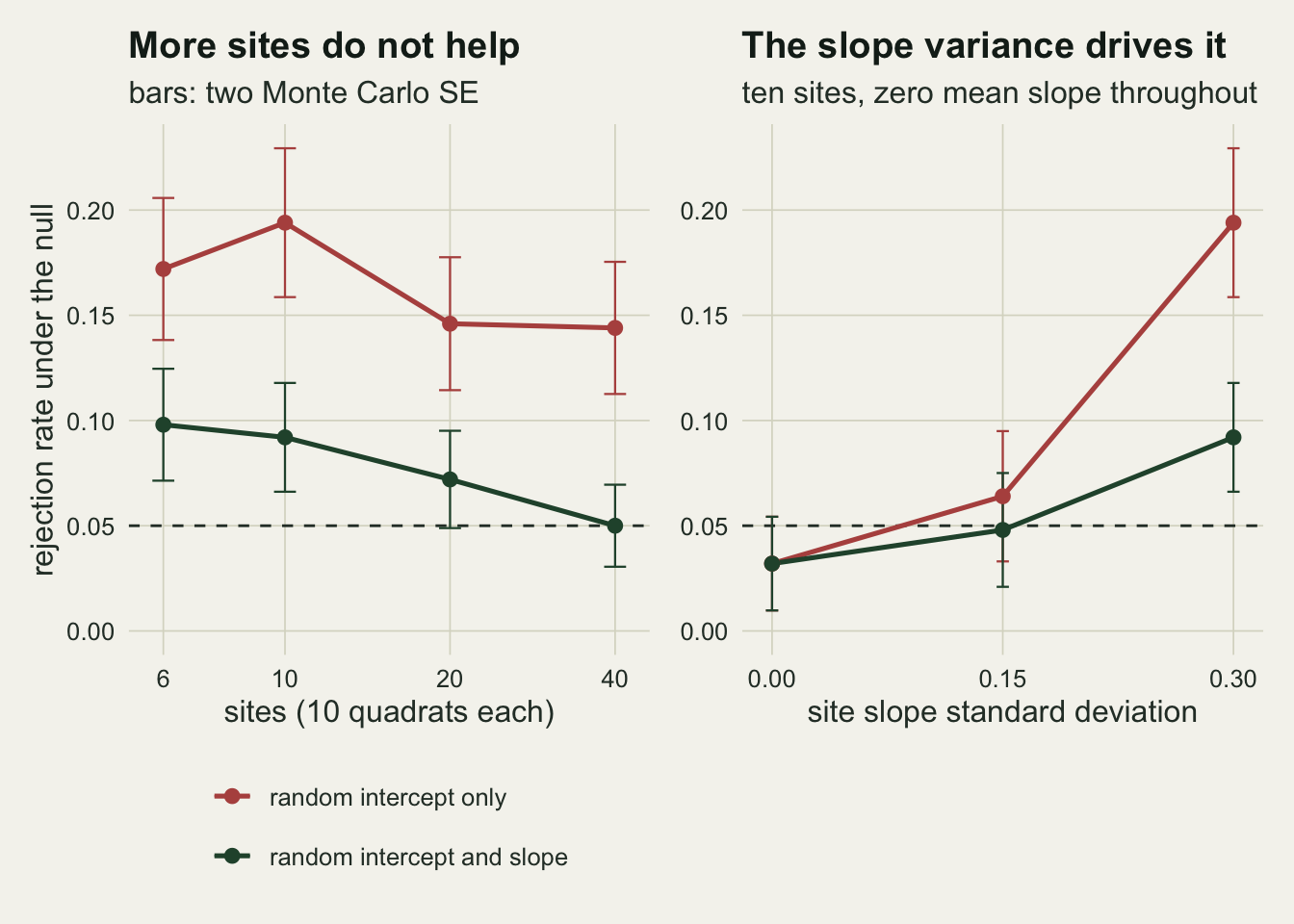
The check fires at its usual rate in the damaged datasets
The defensive workflow is familiar: fit the intercept-only model, test whether a random slope improves it, add the slope if the test says so. The test is a likelihood ratio between the two maximum likelihood fits. Adding a slope variance and its covariance with the intercept puts one parameter on the boundary of its space, so the null distribution of the statistic is an equal mixture of chi squared distributions on one and two degrees of freedom (Stram and Lee 1994), and the five per cent critical value is 5.14 rather than the naive 5.99. The within-site F test, which asks whether separate least squares slopes per site fit better than one common slope, is the second check; it is roughly what an analyst reads off a plot of residuals against the covariate, split by site.
cond_tab <- do.call(rbind, lapply(j_set, function(J) {
  m <- main[main$J == J & !is.na(main$lr), ]
  fp <- m$rej_ri
  do.call(rbind, lapply(c("lrt", "f_fire"), function(chk) {
    fire <- m[[chk]]
    data.frame(J = J, check = chk, state = c("false positive", "no false positive"),
               n = c(sum(fp), sum(!fp)),
               rate = c(mean(fire[fp]), mean(fire[!fp])))
  }))
}))
cond_tab$mcse <- sqrt(cond_tab$rate * (1 - cond_tab$rate) / cond_tab$n)
cond_tab$state <- factor(cond_tab$state, levels = c("false positive", "no false positive"))
cond_tab$check <- factor(ifelse(cond_tab$check == "lrt", "boundary likelihood ratio test",
                                "within-site F test"),
                         levels = c("boundary likelihood ratio test", "within-site F test"))
cd <- function(J, k, s, col = "rate") cond_tab[cond_tab$J == J & as.integer(cond_tab$check) == k &
                                               as.integer(cond_tab$state) == s, col]
diff_lrt <- vapply(j_set, function(J) cd(J, 1, 1) - cd(J, 1, 2), 0)
diff_se  <- vapply(j_set, function(J) sqrt(cd(J, 1, 1, "mcse")^2 + cd(J, 1, 2, "mcse")^2), 0)
diff_z   <- diff_lrt / diff_se

# the other way round: how often the intercept-only result is false, given the check
fp_given <- do.call(rbind, lapply(j_set, function(J) {
  m <- main[main$J == J & !is.na(main$lr), ]
  c(J = J, fire = mean(m$lrt), fp_fire = mean(m$rej_ri[m$lrt]), fp_quiet = mean(m$rej_ri[!m$lrt]))
}))
fg <- function(J, col) fp_given[fp_given[, "J"] == J, col]
With six sites the boundary test fires in 20.2 per cent of all datasets, even though every one of them has a real slope standard deviation of 0.3. With ten sites it fires in 31.2 per cent, twenty 54.0 and forty 82.8. That is the power of the check, and at the small designs typical of field ecology it is low.
The conditional question splits the same datasets by whether the intercept-only model produced a false positive. With six sites the check fires in 15.1 per cent of the 86 false positive datasets and 21.3 per cent of the rest. With ten sites the pair is 29.9 against 31.5 per cent, with twenty 63.0 against 52.5, and with forty 83.3 against 82.7. The differences, in units of their own Monte Carlo standard error, are -1.4, -0.3, 1.7, 0.1 for six, ten, twenty and forty sites: they go both ways and none reaches two. The within-site F test tells the same story: 39.2 against 44.2 per cent at ten sites, 90.3 against 91.6 at forty.
Turned round, this is the statement an analyst can use. With ten sites, when the check fires the intercept-only result is a false positive 18.6 per cent of the time; when the check stays silent, 19.8 per cent of the time. A silent check does not make the intercept-only p value any safer.
ggplot(cond_tab, aes(factor(J), rate, fill = state)) +
  geom_col(position = position_dodge(width = 0.75), width = 0.7, colour = te_paper, linewidth = 0.3) +
  geom_errorbar(aes(ymin = pmax(0, rate - 2 * mcse), ymax = pmin(1, rate + 2 * mcse)),
                position = position_dodge(width = 0.75), width = 0.2, linewidth = 0.4, colour = te_ink) +
  facet_wrap(~ check) +
  scale_fill_manual(values = c(te_rust, te_forest), name = NULL) +
  scale_y_continuous(limits = c(0, 1)) +
  labs(x = "sites", y = "share of datasets in which the check fires",
       title = "The check does not know which datasets went wrong",
       subtitle = "rust: intercept-only model rejected a true zero slope") +
  theme_datasheet() + theme(legend.position = "bottom")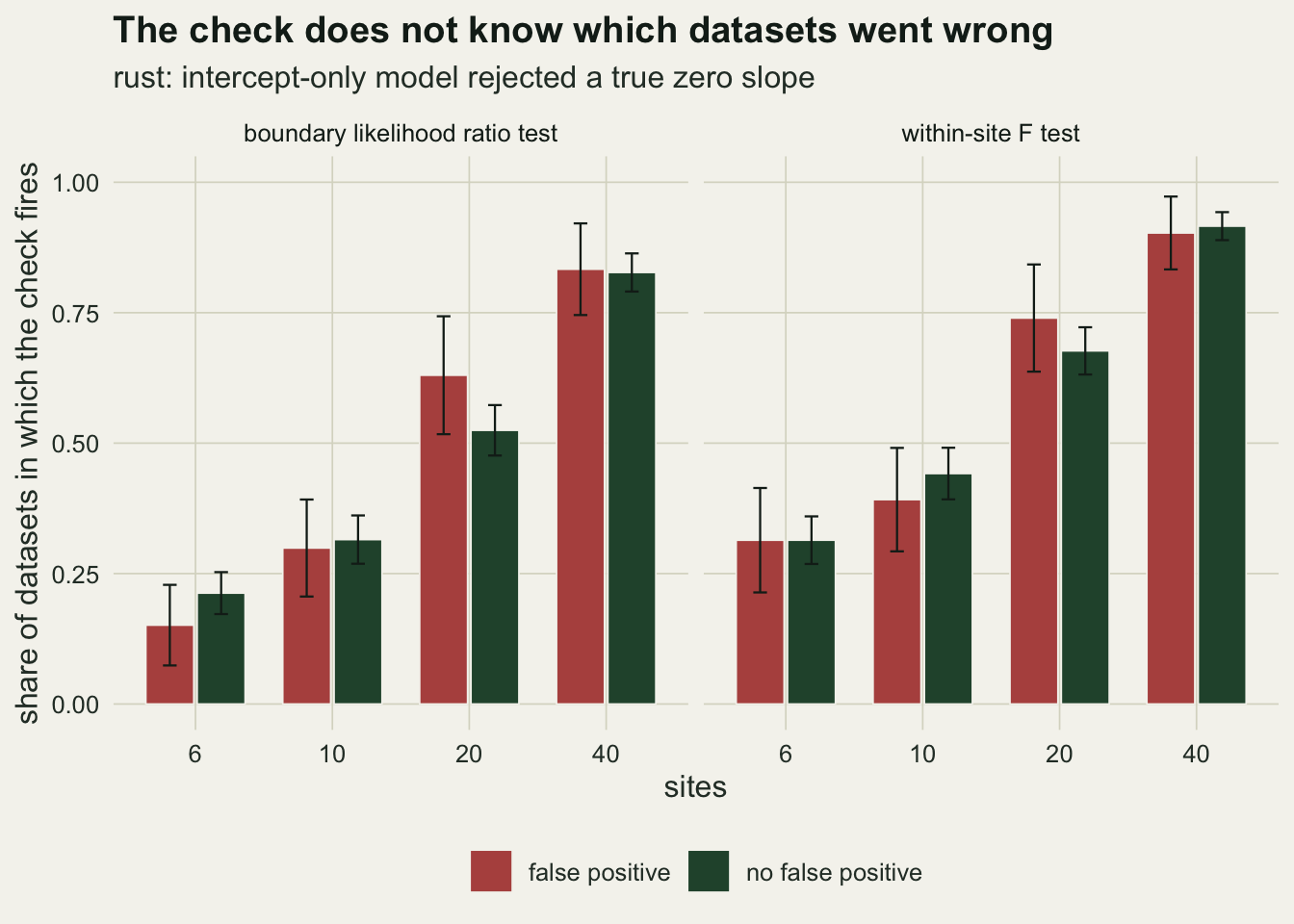
Why the check is blind, and why that was predictable
Nothing about this is surprising once the two statistics are written down. The false positive is driven by the mean of the realised site slopes: if the sampled sites happen to lean one way, the fixed slope estimate leans with them, and the intercept-only standard error does not allow for it. The check is driven by the spread of the realised site slopes. For normally distributed site slopes the sample mean and the sample variance are independent, so a dataset with an unlucky mean is no more likely than any other to have a large spread. The fitted quantities are not exactly those two sample statistics, since the estimates also carry within-site noise, so the independence is approximate.
m10 <- main[main$J == 10 & !is.na(main$lr), ]
vb_fp <- mean(m10$var_b[m10$rej_ri]); vb_ok <- mean(m10$var_b[!m10$rej_ri])
abs_mb_fp <- mean(abs(m10$mean_b[m10$rej_ri])); abs_mb_ok <- mean(abs(m10$mean_b[!m10$rej_ri]))
cor_t_lr <- cor(abs(m10$t_ri), m10$lr, method = "spearman")
cor_mb_vb <- cor(abs(m10$mean_b), m10$var_b, method = "spearman")
crit_ri10 <- qt(1 - alpha_lev / 2, m10$df_ri[1])
With ten sites, the realised variance of the true site slopes averages 0.082 in the false positive datasets and 0.088 in the others, against a generating value of 0.09. The absolute realised mean slope is where they differ: 0.115 against 0.066. The rank correlation between the absolute intercept-only t statistic and the likelihood ratio statistic is 0.000 in absolute value, and between the absolute realised mean and the realised variance of the site slopes 0.045.
m10$outcome <- factor(ifelse(m10$rej_ri, "intercept-only false positive", "no false positive"),
                      levels = c("intercept-only false positive", "no false positive"))
ggplot(m10, aes(lr, abs(t_ri), colour = outcome)) +
  geom_point(size = 1.3, alpha = 0.75) +
  geom_vline(xintercept = crit_mix, colour = te_ink, linetype = "dashed", linewidth = 0.5) +
  geom_hline(yintercept = crit_ri10, colour = te_ink, linetype = "dashed", linewidth = 0.5) +
  scale_x_sqrt(breaks = c(0, 1, 2, 5, 10, 20)) +
  scale_colour_manual(values = c(te_rust, te_forest), name = NULL) +
  labs(x = "likelihood ratio statistic for the random slope (square root axis)",
       y = "absolute t of the fixed slope, intercept-only model",
       title = "Two statistics that ignore each other",
       subtitle = "dashed: five per cent thresholds; right of the vertical line the check fires") +
  theme_datasheet() + theme(legend.position = "bottom")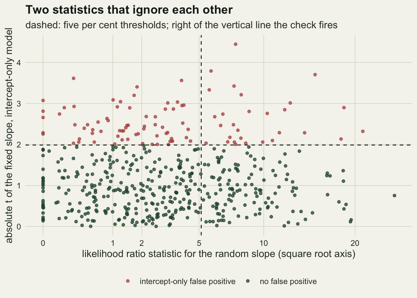
The practical rule follows directly. Whether a covariate that varies within sites gets a random slope has to be decided from the design and the biology, before the data are looked at. It cannot be handed to the test, for two reasons that act together. At six or ten sites the test fires in only 20.2 and 31.2 per cent of datasets that do have a slope variance; and because it answers a question about the spread of the slopes while the false positive is a property of their mean, it fires no more often in the datasets that need it. With many sites the first reason fades, and the second then costs little.
Two repairs and the degrees of freedom
Two repairs are on the table. The maximal model of Barr and colleagues 2013 always includes the random slope. Matuschek and colleagues 2017 argue that this costs power when the slope variance is small, and recommend selecting the random structure with a criterion instead. In their simulations a likelihood ratio test decides at a level of 0.2 rather than 0.05, because 0.05 may penalise the more complex model too strongly. The version here uses the same level, with the boundary mixture as the reference; a plain chi squared reference on two degrees of freedom would keep the slope less often (39.4 against 45.8 per cent of the six-site datasets). Both are applied to the null datasets above, and to one extra set with a real mean slope, to see what the selection buys.
The random slope model’s own excess at small designs needs a word first. nlme gives the fixed moisture slope the degrees of freedom of the within-site level, 53 with six sites, because moisture varies within sites (Pinheiro and Bates 2000). Once the slope is random, the information about its mean comes from the sites, so a reference on the number of sites minus one degrees of freedom is the natural alternative, expected to err on the conservative side. Small-sample corrections of the Kenward-Roger or Satterthwaite kind were not computed here. Kenward-Roger is not implemented for lme fits, and emmeans offers a Satterthwaite option for them. These corrections estimate the degrees of freedom from the variance components, so when the information about the mean slope comes from the sites they should be expected nearer the sites minus one reference than the within-site one; how near, in this design, this page does not measure. The two-stage test (a least squares slope per site, then a one-sample t test on the site slopes) is a third, package-free reference.
set.seed(41209)
n_pow <- 300; b_alt <- 0.2; sd_alt <- 0.15
alt <- sim_cell(n_pow, 10, sd_alt, b_alt)
null_alt <- side[side$J == 10 & side$sd_slope == sd_alt, ]

proc_lev <- c("intercept only", "maximal, lme df", "maximal, sites - 1 df",
              "two-stage site slopes", "select at p < 0.2")
proc_rates <- function(m) c(mean(m$rej_ri), mean(m$rej_rs, na.rm = TRUE),
                            mean(m$rej_rs_j, na.rm = TRUE), mean(m$rej_site), mean(m$rej_sel))
rep_tab <- do.call(rbind, lapply(j_set, function(J)
  data.frame(J = J, procedure = factor(proc_lev, levels = proc_lev),
             rate = proc_rates(main[main$J == J, ]))))
rp <- function(J, k) rep_tab$rate[rep_tab$J == J & as.integer(rep_tab$procedure) == k]
pow_null <- proc_rates(null_alt); pow_alt <- proc_rates(alt)
mcse_pow <- sqrt(0.5 * 0.5 / n_pow)
Under the null with a slope standard deviation of 0.3, the maximal model tested on the sites minus one degrees of freedom rejects at 3.4 per cent with six sites and 4.8 per cent with forty; the two-stage test at 6.4 and 4.6 per cent. The selection rule keeps the slope in 45.8 per cent of the six-site datasets and 94.2 per cent of the forty-site ones, and rejects at 11.2, 11.8, 7.6 and 6.0 per cent over the four designs, above the maximal model with the same degrees of freedom at every design. That is the previous section in another form: the selection drops the slope in datasets chosen at random with respect to the false positives, so it inherits part of the intercept-only error rate.
With six sites the sites minus one reference is at or below nominal and the lme reference is clearly liberal, so at small designs the random slope model’s excess is at least partly a degrees of freedom problem rather than a failure of the random structure. The two-stage test, with no mixed model at all, stays within 1.4 points of nominal across the four designs.
The power comparison uses ten sites, a slope standard deviation of 0.15 and a true mean slope of 0.2. The maximal model with lme degrees of freedom detects it in 49.7 per cent of 300 datasets, the sites minus one version in 40.3, the two-stage test in 43.0 and the selection rule in 55.0 per cent, with a Monte Carlo standard error of at most 2.9 points. At the same slope standard deviation and no mean slope the same four procedures reject at 4.8, 2.4, 3.6 and 5.2 per cent, and the intercept-only model at 6.4 per cent. At this small slope variance the selection rule gained some power for a small cost in false positives, which is the trade Matuschek and colleagues describe; at a slope standard deviation of 0.3 the same rule costs more than the maximal model at every number of sites. Which one wins depends on a variance that the small designs cannot estimate well, which is an argument for deciding on the design grounds before fitting.
ggplot(rep_tab, aes(J, rate, colour = procedure)) +
  geom_hline(yintercept = alpha_lev, colour = te_body, linetype = "dashed", linewidth = 0.5) +
  geom_line(aes(linetype = procedure), linewidth = 0.9) + geom_point(size = 2.2) +
  scale_x_log10(breaks = j_set) +
  scale_colour_manual(values = c(te_rust, te_forest, te_forest, te_gold, "#8a9a8f"), name = NULL) +
  scale_linetype_manual(values = c("solid", "solid", "dashed", "solid", "solid"), name = NULL) +
  scale_y_continuous(limits = c(0, NA)) +
  guides(colour = guide_legend(ncol = 2), linetype = guide_legend(ncol = 2)) +
  labs(x = "sites (10 quadrats each)", y = "rejection rate under the null",
       title = "Repairs and their reference distributions",
       subtitle = "dashed line: the nominal five per cent") +
  theme_datasheet() + theme(legend.position = "bottom")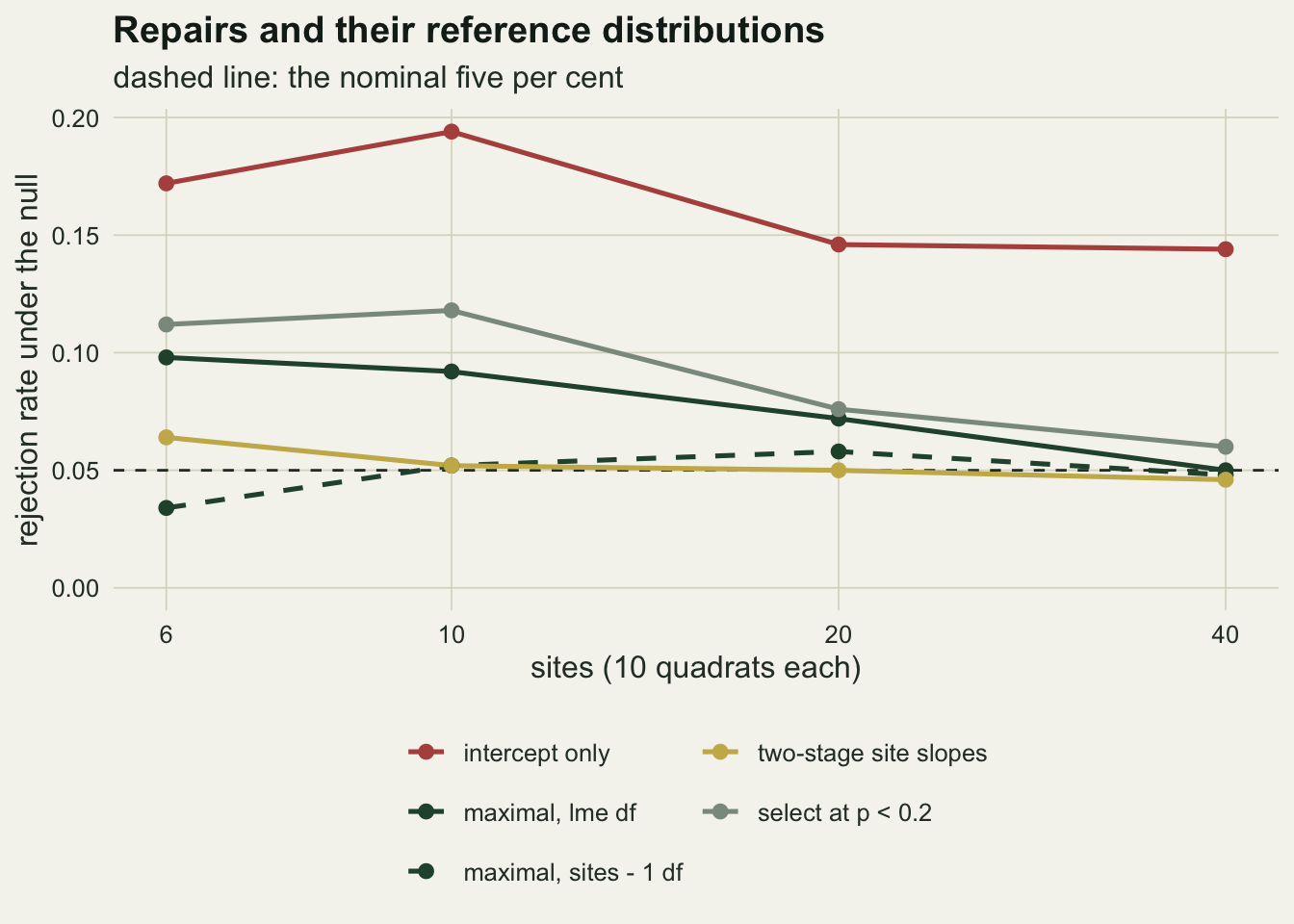
What to report
State whether the covariate varies within the grouping unit, and if it does, whether a random slope was fitted and why. The reason should be the design: sites, individuals or plots that could plausibly respond at different rates. A likelihood ratio test for the slope variance is a legitimate thing to report as a description of the data, but it is not a reason for leaving the slope out.
Report the number of groups next to every fixed slope test, and the degrees of freedom the test used. For a random slope model in nlme those are the within-group degrees of freedom by default, and a reader should know that a test with six sites was referred to a t distribution with dozens of degrees of freedom.
If the random slope was dropped after a test, say so and give the test’s p value and the number of groups. With six or ten sites the test fired in at most a third of datasets that had a real slope standard deviation of 0.3, and the p value from the reduced model does not become more trustworthy because the test was silent.
Where the design is balanced or nearly so, the two-stage estimate (one slope per group, then their mean and its standard error) is a transparent companion to the mixed model. It needs no package and its degrees of freedom are not in question.
Honest limits
Everything here is Gaussian, with ten observations per site, the covariate drawn from the same uniform distribution in every site and no correlation between site intercepts and site slopes. A covariate whose site means differ mixes within- and between-site information about the slope; that is the situation handled by centring in within- and between-individual effects, and it is not simulated here.
Both models are fitted by maximum likelihood, which underestimates variance components in small samples and so makes the random slope model’s own fixed effect test a little liberal. Restricted maximum likelihood changes the variance estimates but not the degrees of freedom nlme assigns, and the sites minus one comparison above suggests the degrees of freedom are the larger part of the excess; it was not run, to keep the post’s run time down.
The selection rule tested is one rule at one level, the level Matuschek and colleagues 2017 used. They compare several criteria over a wider range of slope variances, and their conclusion about power depends on how small the slope variance is; one alternative design here does not settle that trade-off.
The Monte Carlo standard errors of the conditional rates are large, because the false positives are a minority of datasets and each design has only 500 in total. The statement the numbers support is that the check’s firing rate does not depend much on whether the dataset is a false positive; they could not detect a small dependence in either direction.
Kenward-Roger and Satterthwaite corrections were not part of the simulation, so their error rates in this design are not measured here; the reasoning above only leads one to expect them nearer the sites minus one reference than the within-site one. The two-stage test is exact only when every site has the same covariate values.
References
Schielzeth H, Forstmeier W 2009 Behavioral Ecology 20(2):416-420 (10.1093/beheco/arn145)
Barr DJ, Levy R, Scheepers C, Tily HJ 2013 Journal of Memory and Language 68(3):255-278 (10.1016/j.jml.2012.11.001)
Matuschek H, Kliegl R, Vasishth S, Baayen H, Bates D 2017 Journal of Memory and Language 94:305-315 (10.1016/j.jml.2017.01.001)
Stram DO, Lee JW 1994 Biometrics 50(4):1171 (10.2307/2533455)
Pinheiro JC, Bates DM 2000 Mixed-Effects Models in S and S-PLUS (ISBN 978-0-387-98957-0)