library(ggplot2)
library(nlme)

te_paper  <- "#f5f4ee"
te_ink    <- "#16241d"
te_body   <- "#2c3a31"
te_forest <- "#275139"
te_rust   <- "#b5534e"
te_gold   <- "#c9b458"
te_line   <- "#dad9ca"

theme_datasheet <- function() {
  theme_minimal(base_size = 12) +
    theme(plot.background  = element_rect(fill = te_paper, colour = NA),
          panel.background = element_rect(fill = te_paper, colour = NA),
          panel.grid.major = element_line(colour = te_line, linewidth = 0.3),
          panel.grid.minor = element_blank(),
          text             = element_text(colour = te_body),
          plot.title       = element_text(colour = te_ink, face = "bold"),
          plot.subtitle    = element_text(colour = te_body),
          axis.text        = element_text(colour = te_body))
}Within- and between-individual effects in R
R
mixed models
nlme
centring
behavioural ecology
simulation
ecology tutorial
A random intercept slope blends within- and between-female effects. Centring in R with nlme separates them, and why a few records bias the between slope.
A nest-box population of pied flycatchers has been followed for years, and each breeding female carries a ring, so the same bird turns up in the data again and again. For every clutch there is a laying date and a temperature: the mean logger reading at the female’s own box over the fortnight before she laid. The question asked of these data is nearly always the same one. Do females lay earlier when it is warmer?
The temperature has two sources of variation, and the question has two readings. A female that settles in a sheltered, south-facing part of the wood experiences a warmer spring on average than a female on the exposed ridge: that is variation among females. A given female also meets a warmer or colder pre-laying fortnight from one year to the next: that is variation within a female. The biological hypothesis about plasticity, that a bird brings laying forward in a warm spring, is a statement about the within-female part. A comparison among females mixes that response with everything else that differs between the sheltered and the exposed boxes, from caterpillar supply to the age and quality of the birds that win those territories.
The usual model, lme(lay ~ temp, random = ~ 1 | female), returns one slope for temperature. This post measures what that slope is when the within-female and between-female slopes differ, shows the centring fix of van de Pol and Wright (2009) with nlme, and then reproduces a problem that the fix leaves behind, one that the multilevel literature on group means had worked out for contextual effects (Luedtke et al. 2008) and that Westneat et al. (2020) connect, for ecological data, with limited sampling across the range of the covariate: with few records per female, the between-female slope is biased towards the within-female one, even when the true between-female slope is zero.
Several posts on this site sit next to this question without asking it. Behavioural syndromes in R splits a correlation between two behaviours into among-individual and within-individual parts and writes the pooled phenotypic correlation as a mixture of the two; it works with correlations between two responses, not with a slope on a covariate. Random slopes in mixed models with nlme centres its nutrient gradient on the grand mean so that the intercept is interpretable, and never splits the predictor into a group mean and a deviation. Spatial+ and the attenuated slope handles a confounder that varies smoothly in space by taking the residual of the covariate from a spatial smooth; centring on the female mean is the grouped version of that step, with the female factor in place of the smooth and no smoothing parameter to choose. And measurement error and regression dilution shows a noisy predictor pulling a slope towards zero by the reliability ratio; the noisy female mean in the last section obeys the same ratio, but it pulls towards a different target.
Two slopes in one data set
The generating model gives each female a long-run mean temperature, drawn with a standard deviation among females, and adds an independent deviation for each breeding record. Laying date responds to the deviation with a within-female slope of minus two days per degree. It does not respond to the female mean at all: the between-female slope is zero, standing in for a population where warm territories are also poor ones and the two effects cancel. Each female also has her own intercept, a random effect with a standard deviation of two days, and each record has residual noise of three days. All of these constants were fixed before any simulation was run.
b_within  <- -2
b_between <- 0
sd_within <- 1
sd_u      <- 2
sd_e      <- 3
n_fem     <- 100

sim_females <- function(n_fem, n_rec, sd_b, sd_w = sd_within) {
  fem   <- rep(seq_len(n_fem), times = rep_len(n_rec, n_fem))
  m_fem <- rnorm(n_fem, 0, sd_b)
  u_fem <- rnorm(n_fem, 0, sd_u)
  dev   <- rnorm(length(fem), 0, sd_w)
  temp  <- m_fem[fem] + dev
  lay   <- 120 + b_between * m_fem[fem] + b_within * dev +
    u_fem[fem] + rnorm(length(fem), 0, sd_e)
  out <- data.frame(female = factor(fem), temp = temp, lay = lay)
  out$temp_mean <- ave(out$temp, out$female)
  out$temp_dev  <- out$temp - out$temp_mean
  out
}

set.seed(2909)
rec_one <- 5
sdb_one <- 1
one_dat <- sim_females(n_fem, rec_one, sdb_one)
fit_raw <- lme(lay ~ temp, random = ~ 1 | female, data = one_dat)
fit_cen <- lme(lay ~ temp_dev + temp_mean, random = ~ 1 | female, data = one_dat)
fit_mun <- lme(lay ~ temp + temp_mean, random = ~ 1 | female, data = one_dat)

raw_slope   <- fixef(fit_raw)[["temp"]]
cen_within  <- fixef(fit_cen)[["temp_dev"]]
cen_between <- fixef(fit_cen)[["temp_mean"]]
mun_within  <- fixef(fit_mun)[["temp"]]
mun_context <- fixef(fit_mun)[["temp_mean"]]
mun_gap     <- abs(mun_context - (cen_between - cen_within))
raw_ci      <- intervals(fit_raw, which = "fixed")$fixed["temp", c(1, 3)]
In one simulated population of 100 females with 5 records each, and the standard deviation of female mean temperature equal to the within-female one, the uncentred model returns a temperature slope of -1.548 days per degree, with a 95 per cent interval from -1.79 to -1.31. The interval excludes the within-female slope of -2 that generated the data. It excludes the between-female slope of zero as well. It is an estimate of neither.
The centred model replaces temperature with two columns: the female’s mean over her own records, temp_mean, and each record’s deviation from that mean, temp_dev. The two columns are uncorrelated by construction, so adding one does not change the slope of the other. The within-female slope comes out at -1.805 and the between-female slope at -0.700.
Mundlak (1978) wrote the same model a different way: keep the raw temperature and add the female mean as a second covariate. The slope on raw temperature is then the within-female slope, -1.805, identical to the centred fit, and the slope on the mean becomes the contextual effect, the between-female slope minus the within-female slope, 1.105. The two parameterisations agree to 6.66e-16. The Mundlak form is the one to use when the question is whether the two slopes differ, because that difference is a single coefficient with its own standard error.
show_fem  <- levels(one_dat$female)[1:30]
show_dat  <- one_dat[one_dat$female %in% show_fem, ]
fem_means <- aggregate(cbind(temp, lay) ~ female, data = show_dat, FUN = mean)
seg_dat   <- do.call(rbind, lapply(split(show_dat, droplevels(show_dat$female)), function(d_f) {
  x_lo <- min(d_f$temp); x_hi <- max(d_f$temp)
  y_mid <- mean(d_f$lay); x_mid <- mean(d_f$temp)
  data.frame(x0 = x_lo, x1 = x_hi,
             y0 = y_mid + cen_within * (x_lo - x_mid),
             y1 = y_mid + cen_within * (x_hi - x_mid))
}))
grand_x <- mean(one_dat$temp)
grand_y <- mean(one_dat$lay)

ggplot() +
  geom_segment(data = seg_dat, aes(x = x0, xend = x1, y = y0, yend = y1),
               colour = te_forest, linewidth = 0.5, alpha = 0.8) +
  geom_point(data = show_dat, aes(temp, lay), colour = te_forest,
             size = 0.9, alpha = 0.5) +
  geom_point(data = fem_means, aes(temp, lay), colour = te_rust, size = 2.4) +
  geom_abline(intercept = grand_y - cen_between * grand_x, slope = cen_between,
              colour = te_rust, linetype = "dashed", linewidth = 0.8) +
  geom_abline(intercept = grand_y - raw_slope * grand_x, slope = raw_slope,
              colour = te_gold, linewidth = 1.1) +
  labs(x = "pre-laying temperature (deviation from the population mean, deg C)",
       y = "laying date (day of year)",
       title = "Two slopes in one cloud",
       subtitle = "green: within females; red: among female means; gold: the uncentred slope") +
  theme_datasheet()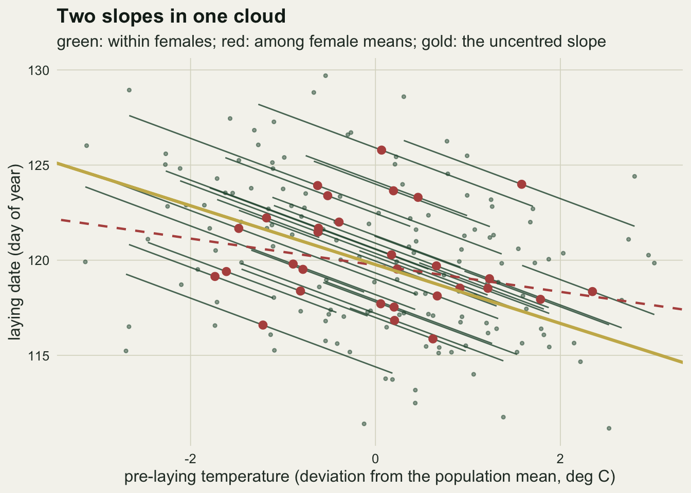
The uncentred slope is a weighted average
For a balanced design, the generalised least squares estimator of a random intercept model is an exact weighted average of two ordinary least squares slopes: the within-female slope, from the deviations, and the between-female slope, from the female means. Maddala (1971) gives the algebra. With W the within sum of squares of temperature, B the between sum of squares (the female means about the grand mean, multiplied by the number of records per female), and theta the ratio of the residual variance to the residual variance plus the number of records times the female variance, the weight on the within slope is W / (W + theta B).
The weight is not a design constant. theta is computed from the variance components the model estimates, and those absorb the part of the data that the single slope cannot fit. The chunk below takes the variance components from the fitted uncentred model, builds the two least squares slopes by hand, and checks the average against lme.
blend_parts <- function(dat, fit) {
  n_rec   <- nrow(dat) / nlevels(dat$female)
  vc      <- as.numeric(VarCorr(fit)[, "Variance"])
  theta   <- vc[2] / (vc[2] + n_rec * vc[1])
  x_bar   <- tapply(dat$temp, dat$female, mean)
  y_bar   <- tapply(dat$lay, dat$female, mean)
  w_xx    <- sum(dat$temp_dev^2)
  b_xx    <- n_rec * sum((x_bar - mean(x_bar))^2)
  slope_w <- sum(dat$temp_dev * (dat$lay - ave(dat$lay, dat$female))) / w_xx
  slope_b <- sum((x_bar - mean(x_bar)) * (y_bar - mean(y_bar))) /
    sum((x_bar - mean(x_bar))^2)
  wt      <- w_xx / (w_xx + theta * b_xx)
  c(weight = wt, slope_w = slope_w, slope_b = slope_b,
    blend = wt * slope_w + (1 - wt) * slope_b)
}

one_parts <- blend_parts(one_dat, fit_raw)
one_gap   <- abs(raw_slope - one_parts[["blend"]])
ols_gap   <- max(abs(c(one_parts[["slope_w"]] - cen_within,
                       one_parts[["slope_b"]] - cen_between)))
The weight on the within-female slope is 0.767. Multiplying it into the two hand-built slopes gives -1.547593, against -1.547593 from lme, a difference of 1.76e-08, of the order of the convergence tolerance of the fitting algorithm. The two hand-built slopes are also the centred model’s slopes, to 6.44e-15: in a balanced design the centred mixed model and two ordinary regressions give the same point estimates.
That identity explains a single fit. To predict the slope before seeing data, the weight has to be written in terms of the generating constants, and the tempting shortcut is to plug the true female and residual variances into theta. That shortcut is wrong, because the fitted model does not see the true variances. Its single slope leaves part of the within-female response in the residual and part of the between-female mismatch in the female intercepts, and the variance estimates grow to hold both. The prediction therefore has to be solved as a fixed point: guess a slope, work out the variances that slope would leave behind, recompute the weight, and repeat. The between-female slope in the prediction is the one the female means actually deliver, which the last section of this post takes apart.
pred_blend <- function(n_rec, sd_b, sd_w = sd_within) {
  lam     <- sd_b^2 / (sd_b^2 + sd_w^2 / n_rec)
  slope_b <- lam * b_between + (1 - lam) * b_within
  w_xx    <- (n_rec - 1) * sd_w^2
  b_xx    <- n_rec * sd_b^2 + sd_w^2
  theta_0 <- sd_e^2 / (sd_e^2 + n_rec * sd_u^2)
  w_naive <- w_xx / (w_xx + theta_0 * b_xx)
  slope   <- slope_b
  for (k in 1:100) {
    v_w   <- sd_e^2 + (b_within - slope)^2 * sd_w^2
    v_b   <- (b_between - slope)^2 * sd_b^2 +
      (b_within - slope)^2 * sd_w^2 / n_rec + sd_u^2 + sd_e^2 / n_rec
    wt    <- w_xx / (w_xx + v_w / (n_rec * v_b) * b_xx)
    slope <- wt * b_within + (1 - wt) * slope_b
  }
  c(lambda = lam, pred_between = slope_b, pred_weight = wt, pred_raw = slope,
    naive_raw = w_naive * b_within + (1 - w_naive) * slope_b)
}
The simulation runs a grid of four record counts per female and three values for the standard deviation of female mean temperature, with the within-female standard deviation fixed at one. Every replicate fits both models with lme and keeps the two slopes, the Wald interval of each against its true value, the blend gap, and a reliability estimate for the female mean that the last section uses.
ci_hit <- function(fit, term, target) {
  tt <- summary(fit)$tTable
  abs(tt[term, "Value"] - target) <= qt(0.975, tt[term, "DF"]) * tt[term, "Std.Error"]
}

rec_grid  <- c(2, 5, 10, 20)
sdb_grid  <- c(0.5, 1, 2)
n_rep     <- 150
cell_grid <- expand.grid(n_rec = rec_grid, sd_b = sdb_grid)

set.seed(4417)
rep_list <- lapply(seq_len(nrow(cell_grid)), function(g) {
  n_rec <- cell_grid$n_rec[g]
  sd_b  <- cell_grid$sd_b[g]
  t(replicate(n_rep, {
    dat   <- sim_females(n_fem, n_rec, sd_b)
    f_raw <- lme(lay ~ temp, random = ~ 1 | female, data = dat)
    f_cen <- lme(lay ~ temp_dev + temp_mean, random = ~ 1 | female, data = dat)
    parts <- blend_parts(dat, f_raw)
    ms_b  <- n_rec * var(tapply(dat$temp, dat$female, mean))
    ms_w  <- sum(dat$temp_dev^2) / (nrow(dat) - n_fem)
    lam_hat <- 1 - ms_w / ms_b
    s_w <- fixef(f_cen)[["temp_dev"]]
    s_b <- fixef(f_cen)[["temp_mean"]]
    c(raw = fixef(f_raw)[["temp"]], within = s_w, between = s_b,
      gap = fixef(f_raw)[["temp"]] - parts[["blend"]],
      hit_raw = ci_hit(f_raw, "temp", b_within),
      hit_within = ci_hit(f_cen, "temp_dev", b_within),
      hit_between = ci_hit(f_cen, "temp_mean", b_between),
      lam_hat = lam_hat,
      corrected = (s_b - (1 - lam_hat) * s_w) / lam_hat)
  }))
})

sim_tab <- do.call(rbind, lapply(seq_along(rep_list), function(g) {
  r_mat <- rep_list[[g]]
  data.frame(cell_grid[g, ],
             raw = mean(r_mat[, "raw"]), raw_se = sd(r_mat[, "raw"]) / sqrt(n_rep),
             within = mean(r_mat[, "within"]),
             between = mean(r_mat[, "between"]),
             between_se = sd(r_mat[, "between"]) / sqrt(n_rep),
             gap = max(abs(r_mat[, "gap"])),
             cov_raw = mean(r_mat[, "hit_raw"]),
             cov_within = mean(r_mat[, "hit_within"]),
             cov_between = mean(r_mat[, "hit_between"]),
             lam_min = min(r_mat[, "lam_hat"]),
             corr_mean = mean(r_mat[, "corrected"]),
             corr_med = median(r_mat[, "corrected"]),
             corr_sd = sd(r_mat[, "corrected"]),
             t(pred_blend(cell_grid$n_rec[g], cell_grid$sd_b[g])))
}))
rownames(sim_tab) <- NULL

cell <- function(n_rec, sd_b, col) sim_tab[sim_tab$n_rec == n_rec & sim_tab$sd_b == sd_b, col]
raw_z     <- (sim_tab$raw - sim_tab$pred_raw) / sim_tab$raw_se
worst_raw <- which.max(abs(raw_z))
naive_off <- max(abs(sim_tab$naive_raw - sim_tab$raw))
naive_row <- which.max(abs(sim_tab$naive_raw - sim_tab$raw))
max_gap   <- max(sim_tab$gap)
mc_cov    <- sqrt(0.95 * 0.05 / n_rep)
raw_diff  <- sim_tab$raw - sim_tab$pred_raw
two_rec   <- sim_tab$n_rec == 2
n_toward  <- sum(raw_diff[two_rec] < 0)
blend_ratio <- cell(20, 0.5, "raw") / cell(2, 2, "raw")
Across all 1800 replicates the largest gap between lme and the weighted average of the two hand-built slopes is 3.18e-07. The identity holds in every fit, not only on average.
The fixed-point prediction tracks the simulation, but not perfectly. At two records per female and equal among- and within-female standard deviations, the mean uncentred slope is -1.265 against a prediction of -1.222; at twenty records it is -1.885 against -1.889. The largest discrepancy in the grid is 0.043 days per degree, or 3.1 Monte Carlo standard errors, at 5 records with a female standard deviation of 2.0. The misses lean one way at the smallest design: in 3 of the 3 cells with two records the simulated slope lies further towards the within-female value than predicted, by up to 0.042. One likely reason is that the prediction puts expected sums of squares and expected variance components into a weight that is a ratio of them, and with few records per female the ratio of expectations is not the expectation of the ratio; the other candidate, noisy REML variance components from two records per female, was not separated from it. The error is small beside the blend itself. The shortcut that plugs in the generating variances misses by up to 0.458 days per degree, in the cell with 10 records and a female standard deviation of 2.0.
blend_plot_dat <- sim_tab
blend_plot_dat$sd_lab <- factor(sprintf("among-female SD %.1f", blend_plot_dat$sd_b),
                                levels = sprintf("among-female SD %.1f", sdb_grid))
sd_cols <- c(te_forest, te_gold, te_rust)

fig_blend <- ggplot(blend_plot_dat, aes(n_rec, raw, colour = sd_lab)) +
  geom_hline(yintercept = c(b_within, b_between), linetype = "dashed",
             colour = te_body, linewidth = 0.5) +
  geom_line(aes(y = pred_raw), linewidth = 0.9) +
  geom_errorbar(aes(ymin = raw - 2 * raw_se, ymax = raw + 2 * raw_se),
                width = 0.04, linewidth = 0.6) +
  geom_point(size = 2.6) +
  scale_x_log10(breaks = rec_grid) +
  scale_colour_manual(values = sd_cols, name = NULL) +
  annotate("text", x = 2, y = b_within, label = "within-female slope",
           vjust = -0.6, hjust = 0, colour = te_body, size = 3.4) +
  annotate("text", x = 2, y = b_between, label = "between-female slope",
           vjust = 1.6, hjust = 0, colour = te_body, size = 3.4) +
  labs(x = "records per female (log scale)",
       y = "uncentred slope (days per deg C)",
       title = "The single slope is a blend",
       subtitle = "points: simulation; lines: fixed-point prediction") +
  theme_datasheet() +
  theme(legend.position = "bottom")
fig_blend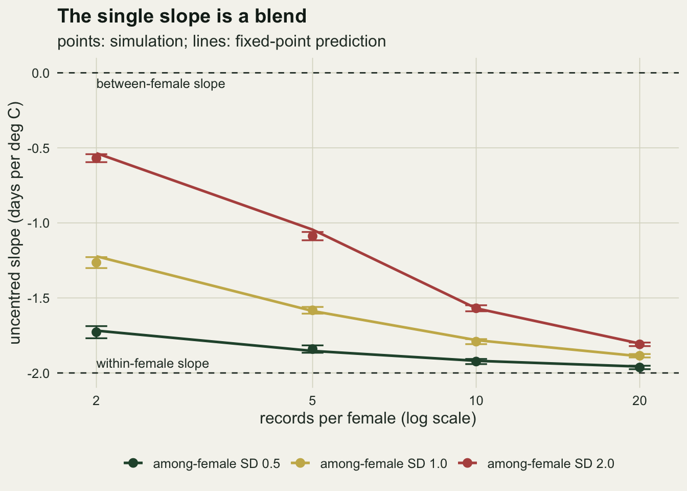
The figure carries the practical message of this section. The uncentred slope depends on the design as much as on the biology. With the same within-female response of -2 days per degree, a study whose territories differ widely in temperature and which has 2 records per female reports -0.57, and a study with narrow territorial differences and 20 records per female reports -1.96. Two populations with the same plasticity can publish slopes that differ by a factor of 3.5.
Centring recovers the within slope and its interval
The Wald interval of the uncentred slope is built for a slope that is neither of the two true ones, so its coverage of the within-female slope is whatever the blend allows. At two records per female and equal standard deviations the interval covers -2 in 0.073 of replicates. With a female standard deviation of two it covers in 0.000 at two records and 0.187 at twenty.
cov_within_all <- mean(sim_tab$cov_within)
cov_within_min <- min(sim_tab$cov_within)
cov_within_row <- which.min(sim_tab$cov_within)
cov_pool_se    <- sqrt(cov_within_all * (1 - cov_within_all) / (nrow(sim_tab) * n_rep))
cov_pool_z     <- (0.95 - cov_within_all) / sqrt(0.95 * 0.05 / (nrow(sim_tab) * n_rep))
cov_min_z      <- (0.95 - cov_within_min) / mc_cov
cov_next_z     <- (0.95 - sort(sim_tab$cov_within)[2]) / mc_cov
within_bias    <- max(abs(sim_tab$within - b_within))
The centred model’s within-female slope has a largest mean bias of 0.019 across the grid. Its interval covers the true value in 0.943 of all replicates pooled, with a Monte Carlo standard error of 0.005. That pooled rate is 1.4 standard errors below the nominal level. The lowest single cell, 0.900 at 5 records with a female standard deviation of 0.5, is 2.8 cell standard errors of 0.018 below it; the smallest of twelve cells is expected to sit low, and the next lowest is 1.7 below. The simulation cannot tell a slightly liberal interval at few records from chance.
cov_long <- rbind(
  data.frame(sim_tab[, c("n_rec", "sd_b")], coverage = sim_tab$cov_raw,
             interval = "uncentred slope, target -2"),
  data.frame(sim_tab[, c("n_rec", "sd_b")], coverage = sim_tab$cov_within,
             interval = "centred within slope, target -2"),
  data.frame(sim_tab[, c("n_rec", "sd_b")], coverage = sim_tab$cov_between,
             interval = "centred between slope, target 0"))
cov_long$interval <- factor(cov_long$interval, levels = unique(cov_long$interval))
cov_long$sd_lab <- factor(sprintf("among-female SD %.1f", cov_long$sd_b),
                          levels = sprintf("among-female SD %.1f", sdb_grid))

ggplot(cov_long, aes(n_rec, coverage, colour = interval)) +
  geom_hline(yintercept = 0.95, linetype = "dashed", colour = te_body, linewidth = 0.5) +
  geom_line(linewidth = 0.8) +
  geom_point(size = 2.2) +
  facet_wrap(~ sd_lab, nrow = 1) +
  scale_x_log10(breaks = rec_grid) +
  scale_colour_manual(values = c(te_gold, te_forest, te_rust), name = NULL) +
  labs(x = "records per female (log scale)", y = "coverage",
       title = "Only the centred within slope keeps its interval",
       subtitle = "150 replicates per point") +
  theme_datasheet() +
  theme(legend.position = "bottom", legend.direction = "vertical",
        panel.spacing = unit(1.2, "lines"))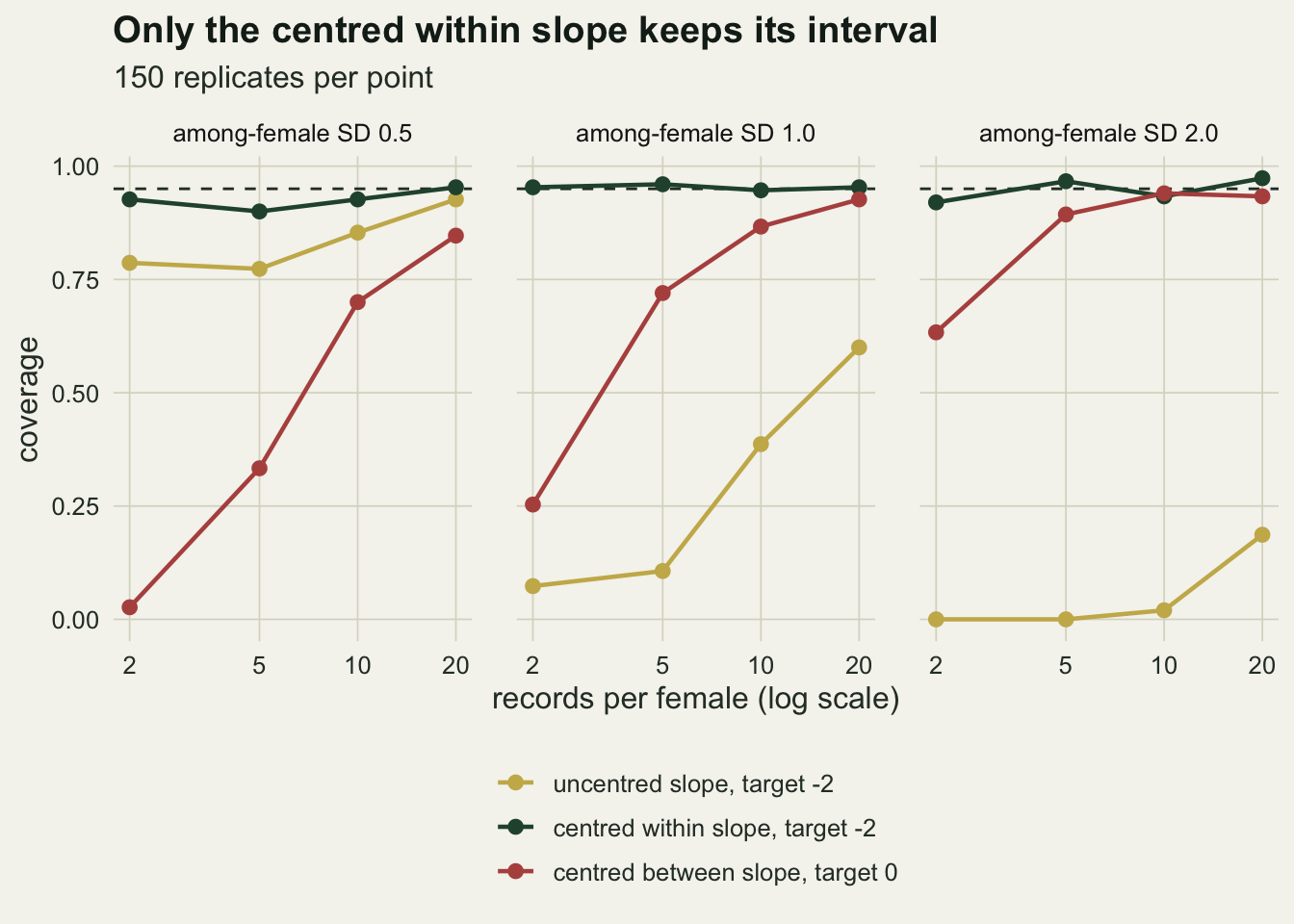
The rust line in that figure is the subject of the next section. The between-female slope was generated as zero, and the centred model’s interval for it misses zero far more often than five times in a hundred when records per female are few.
The female mean is a noisy covariate
The centred model regresses on the female mean over her sampled records, not on her long-run mean. With n records the sampled mean is the long-run mean plus an average of n within-female deviations, and those deviations are exactly the quantity laying date responds to with a slope of -2. The average of the deviations does not vanish at small n, so the female means carry a piece of the within-female response, and the regression on them picks it up.
Write lambda for the reliability of the sampled mean, the share of its variance that is long-run among-female variance: the among-female variance divided by that variance plus the within-female variance over n. The covariance of female mean laying date with female mean temperature is the between slope times the among-female variance plus the within slope times the within-female variance over n. Dividing by the variance of the sampled mean gives an expected between-female estimate of lambda times the true between slope plus one minus lambda times the true within slope. This is the reliability ratio from classical measurement error, with one change: the error in the female mean is correlated with the response, so the estimate is pulled towards the within-female slope rather than towards zero. When the true within slope is zero the two stories coincide. Neither the bias nor the correction below is new: Luedtke et al. (2008) derive the bias in contextual effects estimated from observed group means in multilevel models, with the reliability of the group mean in exactly this role, and fit a latent covariate model that removes it, and Westneat et al. (2020) report biased parameters in mean-centred analyses of ecological data when sampling across the range of the covariate is limited. This section reproduces them by simulation.
att_z     <- (sim_tab$between - sim_tab$pred_between) / sim_tab$between_se
worst_att <- which.max(abs(att_z))
ctx_true  <- b_between - b_within
ctx_two   <- cell(2, 1, "between") - cell(2, 1, "within")
ctx_twenty <- cell(20, 1, "between") - cell(20, 1, "within")
At two records per female and equal standard deviations lambda is 0.667, and the prediction for the between-female slope is -0.667. The simulation returns -0.718. With a female standard deviation of one half, lambda falls to 0.333 and the between-female slope averages -1.351 against a prediction of -1.333; the true value is still zero. The largest discrepancy from the prediction in the grid is 2.5 Monte Carlo standard errors, at 2 records and a female standard deviation of 2.0.
The consequence for inference is the rust line in the coverage figure. At two records and equal standard deviations the interval for the between-female slope contains zero in 0.253 of replicates, so a study of this design reports a between-female temperature effect in most replicates where none exists. The false effect has the same sign as the real within-female one, which makes it look like corroboration.
lam_line <- data.frame(lambda = seq(0.3, 1, length.out = 100))
lam_line$pred <- lam_line$lambda * b_between + (1 - lam_line$lambda) * b_within
betw_dat <- sim_tab
betw_dat$rec_lab <- factor(sprintf("%d records", betw_dat$n_rec),
                           levels = sprintf("%d records", rec_grid))

ggplot(betw_dat, aes(lambda, between)) +
  geom_hline(yintercept = b_between, linetype = "dashed", colour = te_body, linewidth = 0.5) +
  geom_line(data = lam_line, aes(lambda, pred), colour = te_ink, linewidth = 0.8) +
  geom_errorbar(aes(ymin = between - 2 * between_se, ymax = between + 2 * between_se,
                    colour = rec_lab), width = 0.012, linewidth = 0.6) +
  geom_point(aes(colour = rec_lab), size = 2.6) +
  scale_colour_manual(values = c(te_rust, te_gold, te_forest, te_ink), name = NULL) +
  labs(x = "reliability of the sampled female mean (lambda)",
       y = "between-female slope (days per deg C)",
       title = "The female mean borrows the within slope",
       subtitle = "true between-female slope: zero (dashed)") +
  theme_datasheet() +
  theme(legend.position = "bottom")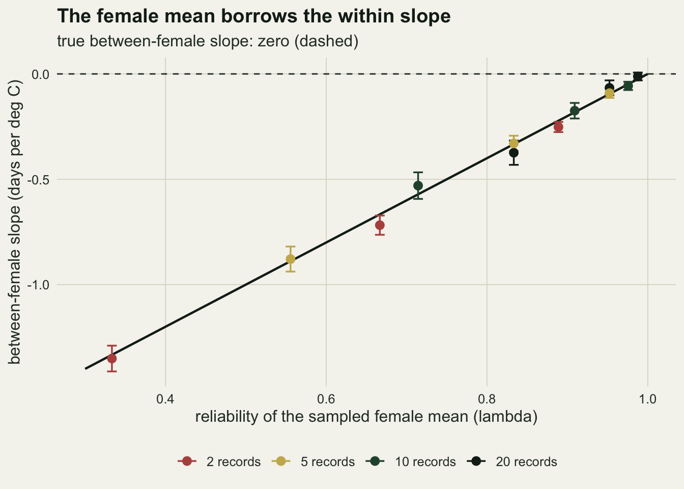
Because each female has several records, lambda can be estimated from the covariate alone, using the one-way mean squares of temperature by female: one minus the within mean square over the between mean square. This is a moment-based reliability correction for an observed group mean, the adjustment that the latent covariate model of Luedtke et al. (2008) makes inside the fit: the between slope is corrected by subtracting one minus that estimate times the within slope and dividing by the estimate. The chunk that ran the grid already kept the corrected value for every replicate.
At two records and equal standard deviations the corrected between-female slope averages -0.024, with a standard deviation across replicates of 0.496, against -0.718 uncorrected. The correction fails where it is needed most. With a female standard deviation of one half and two records, the smallest estimated lambda among the replicates is -0.249, a negative estimate, which flips the sign of the correction; the corrected slope averages 0.822 with a standard deviation of 6.51, and only its median, -0.027, sits near zero. Even where the correction centres near zero, at two records and equal standard deviations, its replicate standard deviation of 0.496 is the price. Dividing by a small, noisy reliability is the same instability that the measurement error post describes, and here it arrives exactly when females contribute only two records and differ little in their mean conditions.
What to report
Report the within-individual and between-individual slopes separately, from a centred or a Mundlak model, and give the number of records per individual next to them. A single slope from a random intercept model on an uncentred covariate is a weighted average whose weight depends on the number of records and the spread of individual means, so it cannot be compared between studies, and in the grid here the same within-female response produced slopes from -1.96 to -0.57.
State the question the slope answers. Plasticity, the change within an individual, is the within slope. The between slope compares individuals and inherits everything else that differs among them: territory, age, quality, and which birds survive to contribute several records. It is a description of the population, and in an observational study it is not an estimate of what warming would do to any one female.
When the between slope matters, report the reliability of the individual mean for the covariate, estimated from the one-way mean squares. If it is well below one, the between slope is pulled towards the within slope by one minus the reliability, and a between slope that looks like confirmation of the within slope may be an artefact of the design.
Van de Pol and Wright (2009) give the centring recipe in the form used here. Dingemanse and Dochtermann (2013) set out the matching split for variances and correlations, between individuals and within them, together with the sampling designs that estimate each; the slope split belongs in the same table. Use the Mundlak coefficient on the individual mean, with its interval, when the question is whether the two slopes differ. It is the same model as the centred one, and it inherits the noisy-mean problem of the last section: its expected value is approximately the reliability times the true difference. At two records and equal standard deviations the true difference of 2 comes out on average as 1.284, and at twenty records as 1.929, so with few records per individual the test understates the difference.
Honest limits
The design is balanced: every female has the same number of records. That is what makes the weighted average exact with a single weight. With unequal numbers of records each female’s mean has its own reliability and each female gets her own weight in the generalised least squares estimator, so the scalar formula in the blend chunk becomes an approximation. Only one unbalanced population was run, so the grid results above are claimed for balanced data only.
set.seed(6021)
rec_unbal <- sample(2:10, n_fem, replace = TRUE)
unbal_dat <- sim_females(n_fem, rec_unbal, sdb_one)
fit_unbal <- lme(lay ~ temp, random = ~ 1 | female, data = unbal_dat)
unbal_gap <- abs(fixef(fit_unbal)[["temp"]] - blend_parts(unbal_dat, fit_unbal)[["blend"]])
One simulated population with between two and ten records per female shows the size of that approximation: the scalar formula, with the mean number of records in place of a constant, misses the lme slope by 0.0069, against 1.76e-08 in the balanced fit.
The within-female deviations are independent across records and across females. A real pre-laying temperature has a strong year component shared by every female breeding that year, and the year also affects laying date through routes other than temperature. In that case the within-female deviations are confounded with year, a crossed year random effect or year fixed effects are needed, and the within-female slope from this post’s model would absorb any year effect that runs with temperature.
The between-female bias is defined against the female’s long-run mean. If the biological effect runs through the temperatures a female actually experienced in the years she bred, then her sampled mean is the right covariate, it is not noisy, and there is nothing to correct; this mismatch between the generating process and the centred model is the central point of Westneat et al. (2020). Which mean is the right one is a question about the biology, not the statistics, and the answer decides whether the last section applies.
No random slope was simulated or fitted. Every female responds with the same within-female slope, so the within-female interval kept its coverage without one. When females differ in plasticity, the within-female interval from a random intercept model is too narrow, which is the point made in the random slopes post, and the centred model needs a random slope on the deviation to keep it.
The response is Gaussian with constant variance. In a generalised linear mixed model the centring still separates the two slopes, but the weighted average is no longer an exact identity, and the reliability argument for the between slope was not checked on a link scale.
References
van de Pol M, Wright J 2009 Animal Behaviour 77(3):753-758 (10.1016/j.anbehav.2008.11.006)
Mundlak Y 1978 Econometrica 46(1):69-85 (10.2307/1913646)
Luedtke O, Marsh HW, Robitzsch A, Trautwein U, Asparouhov T, Muthen B 2008 Psychological Methods 13(3):203-229 (10.1037/a0012869)
Maddala GS 1971 Econometrica 39(2):341-358 (10.2307/1913349)
Dingemanse NJ, Dochtermann NA 2013 Journal of Animal Ecology 82(1):39-54 (10.1111/1365-2656.12013)
Westneat DF, Araya-Ajoy YG, Allegue H, Class B, Dingemanse N, Dochtermann NA, Garamszegi LZ, Martin JGA, Nakagawa S, Reale D, Schielzeth H 2020 Journal of Animal Ecology 89(12):2813-2824 (10.1111/1365-2656.13360)