library(ggplot2)
library(patchwork)
library(mgcv)

te_paper  <- "#f5f4ee"
te_ink    <- "#16241d"
te_body   <- "#2c3a31"
te_forest <- "#275139"
te_rust   <- "#b5534e"
te_gold   <- "#c9b458"
te_line   <- "#dad9ca"

theme_datasheet <- function() {
  theme_minimal(base_size = 12) +
    theme(plot.background  = element_rect(fill = te_paper, colour = NA),
          panel.background = element_rect(fill = te_paper, colour = NA),
          panel.grid.major = element_line(colour = te_line, linewidth = 0.3),
          panel.grid.minor = element_blank(),
          text             = element_text(colour = te_body),
          plot.title       = element_text(colour = te_ink, face = "bold"),
          plot.subtitle    = element_text(colour = te_body),
          axis.text        = element_text(colour = te_body))
}Spatial+ and the attenuated slope
R
GAMs
mgcv
spatial
spatial confounding
simulation
ecology tutorial
Adding a spatial smooth to a GAM moves a confounded slope only part of the way back. Spatial+ in R with mgcv, and the plot-level variation it needs to work.
Three hundred vegetation plots are scattered over a ten by ten kilometre reserve. In each one somebody measured soil pH and the log cover of a calcicole herb, and the question is how steeply cover rises with pH. Soil pH has two sources of variation. Part of it follows the bedrock and changes slowly across the map; part of it is local, a limestone boulder here, a pocket of acid litter there, and changes from one plot to the next. The herb also responds to something nobody measured, a broad legacy of past grazing that happens to run against the bedrock gradient, so the plots with the most alkaline bedrock were also the ones grazed hardest.
A plain regression of cover on pH mixes the pH effect with the grazing legacy. The textbook reflex is to add a smooth of the coordinates, s(lon, lat), and let it take up whatever varies smoothly in space. The post on checking a spatial regression measured the diagnosis of what happens next, under the heading “The honest limit: spatial confounding”: as eigenvector maps entered a regression with a smooth covariate, the variance inflation factor of the covariate climbed and its standard error nearly tripled. It closed with the restricted spatial regression of Hodges and Reich, noted that whether it is the right choice depends on the question, and said plainly that “there is no universal fix”.
This post writes one fix out in full and measures it. Spatial+ (Dupont, Wood and Augustin 2022) is two ordinary mgcv fits: smooth the covariate on the coordinates, keep its residual, and use that residual in place of the covariate in the spatial model. It is not universal either, and the last simulation section shows where it stops helping. The companion posts are concurvity in additive models, which is the same identifiability problem between two smooth terms, and generalised least squares for spatial data, which repairs the standard error when spatial structure sits only in the residual and nothing is confounded.
Three hundred plots on one map
The generating model has a covariate made of a smooth field plus independent plot-level noise, and a response that adds a second smooth field correlated with the first. Every field is a Gaussian random field with unit variance and a squared exponential correlation that falls to about a third at three kilometres, so the fields vary on the scale of the whole reserve. All the constants below were fixed before any simulation was run.
n_plot   <- 300      # vegetation plots
map_km   <- 10       # side of the reserve
range_km <- 3        # correlation length of every smooth field
beta_set <- 1        # true slope of log cover on pH (standardised units)
r_conf   <- -0.6     # correlation of the grazing legacy with the bedrock field
sd_local <- 0.5      # sd of plot-level pH variation (bedrock field sd is one)
sd_noise <- 1        # residual sd of log cover
k_sp     <- 50       # basis dimension of s(lon, lat)
z95      <- qnorm(0.975)

set.seed(2204)
plots <- data.frame(lon = runif(n_plot, 0, map_km), lat = runif(n_plot, 0, map_km))
dist_km <- as.matrix(dist(plots))
chol_field <- t(chol(exp(-(dist_km / range_km)^2) + diag(1e-6, n_plot)))
draw_field <- function() as.vector(chol_field %*% rnorm(n_plot))

draw_reserve <- function(r = r_conf, sd_x = sd_local) {
  bedrock <- draw_field()
  grazing <- r * bedrock + sqrt(1 - r^2) * draw_field()
  ph      <- bedrock + rnorm(n_plot, 0, sd_x)
  cover   <- beta_set * ph + grazing + rnorm(n_plot, 0, sd_noise)
  data.frame(plots, ph = ph, cover = cover, bedrock = bedrock, grazing = grazing)
}
share_local <- sd_local^2 / (1 + sd_local^2)
The plots stay where they are in every replicate; only the fields and the noise are redrawn. With these constants 20 per cent of the variance in pH is plot-level variation that has nothing to do with the map, and the grazing legacy correlates at -0.6 with the bedrock part of pH.
set.seed(517)
res1 <- draw_reserve()
fit_ols  <- lm(cover ~ ph, data = res1)
fit_gam  <- gam(cover ~ ph + s(lon, lat, k = k_sp), data = res1, method = "REML")
fit_phsp <- gam(ph ~ s(lon, lat, k = k_sp), data = res1, method = "REML")
res1$ph_spatial <- fitted(fit_phsp)
res1$ph_resid   <- residuals(fit_phsp)
fit_plus <- gam(cover ~ ph_resid + s(lon, lat, k = k_sp), data = res1, method = "REML")

slope_row <- function(est, se) c(est = unname(est), lo = unname(est - z95 * se), hi = unname(est + z95 * se))
w_tab <- rbind(ols  = slope_row(coef(fit_ols)["ph"], summary(fit_ols)$coefficients["ph", 2]),
               gam  = slope_row(coef(fit_gam)["ph"], sqrt(vcov(fit_gam)["ph", "ph"])),
               plus = slope_row(coef(fit_plus)["ph_resid"], sqrt(vcov(fit_plus)["ph_resid", "ph_resid"])))
cor_resid_bed <- cor(res1$ph_resid, res1$bedrock)
cor_ph_graz   <- cor(res1$ph, res1$grazing)
cor_resid_graz <- cor(res1$ph_resid, res1$grazing)
edf_phsp <- sum(fit_phsp$edf)
resid_share1 <- var(res1$ph_resid) / var(res1$ph)
round(w_tab, 3)
est lo hi
ols 0.556 0.450 0.662
gam 1.040 0.826 1.255
plus 1.142 0.891 1.393On this one reserve the plain regression puts the slope at 0.56 (interval 0.45 to 0.66), the spatial GAM at 1.04 (0.83 to 1.25) and spatial+ at 1.14 (0.89 to 1.39), against a true value of 1. On this reserve the spatial GAM happens to land nearer the truth than spatial+, which is what one draw can do; the next section asks what happens on average.
The first stage of spatial+ is the smooth of pH on the coordinates, which here uses 37.0 effective degrees of freedom. Raw pH correlates at -0.69 with the grazing legacy; its residual after the smooth correlates at -0.02, and at 0.04 with the bedrock field it came from. The residual keeps 11 per cent of the variance of pH, and it is what the second stage estimates the slope from.
map_panel <- function(value, title) {
  lim <- max(abs(value))
  ggplot(res1, aes(lon, lat, colour = value)) +
    geom_point(size = 1.6) +
    scale_colour_gradient2(low = te_rust, mid = te_line, high = te_forest,
                           midpoint = 0, limits = c(-lim, lim), name = NULL) +
    coord_equal() +
    labs(x = "km east", y = "km north", title = title) +
    theme_datasheet() +
    theme(legend.position = "bottom", legend.key.width = unit(0.6, "cm"),
          plot.title = element_text(size = 11))
}
map_panel(res1$ph, "pH as measured") +
  map_panel(res1$ph_spatial, "smooth part") +
  map_panel(res1$ph_resid, "residual pH") +
  plot_annotation(theme = theme_datasheet())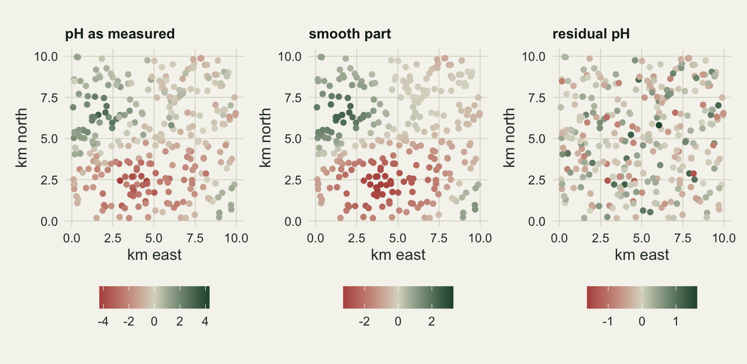
The spatial GAM moves the slope part of the way
One reserve is one draw. The simulation repeats the three analyses on freshly drawn fields. The thin plate regression spline basis for s(lon, lat) (Wood 2017) depends only on the plot coordinates, which never change, so the model matrices are built once with fit = FALSE and each replicate swaps in the new response and covariate before calling gam(). The worked fit above is refitted through the same shortcut as a check.
g_cover <- gam(cover ~ ph + s(lon, lat, k = k_sp), data = res1, method = "REML", fit = FALSE)
g_ph    <- gam(ph ~ s(lon, lat, k = k_sp), data = res1, method = "REML", fit = FALSE)
refit <- function(g, yy, xcol = NULL) {
  g$y <- yy; g$mf[[1]] <- yy
  if (!is.null(xcol)) g$X[, 2] <- xcol
  gam(G = g, method = "REML")
}
chk_gap <- max(abs(c(coef(refit(g_cover, res1$cover, res1$ph)) - coef(fit_gam),
                     residuals(refit(g_ph, res1$ph)) - res1$ph_resid,
                     coef(refit(g_cover, res1$cover, res1$ph_resid)) - coef(fit_plus))))

one_rep <- function(r = r_conf, sd_x = sd_local) {
  d <- draw_reserve(r, sd_x)
  ols <- summary(lm(cover ~ ph, data = d))$coefficients["ph", 1:2]
  m_gam <- refit(g_cover, d$cover, d$ph)
  ph_r  <- residuals(refit(g_ph, d$ph))
  m_plus <- refit(g_cover, d$cover, ph_r)
  c(ols[1], coef(m_gam)[2], coef(m_plus)[2],
    ols[2], sqrt(vcov(m_gam)[2, 2]), sqrt(vcov(m_plus)[2, 2]),
    var(ph_r) / var(d$ph))
}
method_lev <- c("plain regression", "spatial GAM", "spatial+")
summarise_reps <- function(reps, scenario) {
  est <- reps[, 1:3, drop = FALSE]; se <- reps[, 4:6, drop = FALSE]
  covered <- abs(est - beta_set) <= z95 * se
  data.frame(scenario = scenario, method = factor(method_lev, levels = method_lev),
             mean_est = colMeans(est), sd_est = apply(est, 2, sd),
             mean_se = colMeans(se), coverage = colMeans(covered),
             width = colMeans(2 * z95 * se), resid_share = mean(reps[, 7]),
             n_rep = nrow(reps), row.names = NULL)
}
The shortcut reproduces the direct fits: the largest absolute difference across the coefficients and first-stage residuals is 0.0e+00, so the two routes are the same computation.
n_rep_main <- 250   # fixed before any result was seen
set.seed(9031)
reps_conf <- t(replicate(n_rep_main, one_rep()))
tab_conf <- summarise_reps(reps_conf, "grazing confounded")
at <- function(tab, m, col) tab[tab$method == method_lev[m], col]
mcse_mean <- function(tab, m) at(tab, m, "sd_est") / sqrt(at(tab, m, "n_rep"))
mcse_cov95 <- sqrt(0.95 * 0.05 / n_rep_main)
gam_share_back <- (at(tab_conf, 2, "mean_est") - at(tab_conf, 1, "mean_est")) /
                  (beta_set - at(tab_conf, 1, "mean_est"))
plus_bias_z <- (at(tab_conf, 3, "mean_est") - beta_set) / mcse_mean(tab_conf, 3)
tab_conf[, c("method", "mean_est", "sd_est", "mean_se", "coverage")]
method mean_est sd_est mean_se coverage
1 plain regression 0.5495525 0.2172505 0.07384559 0.088
2 spatial GAM 0.8699727 0.1180832 0.10497267 0.688
3 spatial+ 1.0332871 0.1217399 0.12440257 0.944Over 250 reserves the plain regression averages 0.550, the spatial GAM 0.870 and spatial+ 1.033, with Monte Carlo standard errors of 0.014, 0.007 and 0.008. The grazing legacy pulls the plain slope down, and adding the smooth recovers 71 per cent of the gap to the truth and no more. Spatial+ is not exactly unbiased either: its mean sits 0.033 above the truth, 4.3 Monte Carlo standard errors, which is small next to the spread of a single estimate but is not simulation noise. A later section takes that bias apart.
Coverage of the nominal 95 per cent interval is 0.088 for the plain regression, 0.688 for the spatial GAM and 0.944 for spatial+, where a correct interval would sit within about 0.028 of 0.95.
Why the smooth does not finish the job is the point of the Dupont, Wood and Augustin paper. The bedrock part of pH is itself a smooth function of the coordinates, so the covariate and s(lon, lat) compete for the same variation, the problem the concurvity post describes. The smoothing penalty makes the spatial term the more expensive of the two, and the fit hands part of the grazing signal to the unpenalised pH coefficient. How much it hands over depends on the smoothing parameter, which is chosen for the fit of the whole surface, not for the slope. Spatial+ removes the competition: its covariate has had the smooth part taken out, so what is left for the slope is mostly the plot-level variation, which the grazing legacy cannot touch. Mostly, because a penalised smooth leaves a little of the smooth part behind, and that remainder is where the small upward bias of spatial+ comes from.
est_long <- data.frame(method = factor(rep(method_lev, each = n_rep_main), levels = method_lev),
                       est = as.vector(reps_conf[, 1:3]))
ggplot(est_long, aes(method, est, colour = method)) +
  geom_hline(yintercept = beta_set, colour = te_body, linetype = "dashed", linewidth = 0.5) +
  geom_jitter(width = 0.18, height = 0, alpha = 0.45, size = 1.3) +
  geom_point(data = tab_conf, aes(method, mean_est), colour = te_ink, size = 3.2, shape = 18) +
  scale_colour_manual(values = c(te_rust, te_gold, te_forest), guide = "none") +
  labs(x = NULL, y = "estimated slope of log cover on pH",
       title = "The smooth moves the slope, spatial+ moves it back",
       subtitle = "dark diamonds: mean over reserves") +
  theme_datasheet()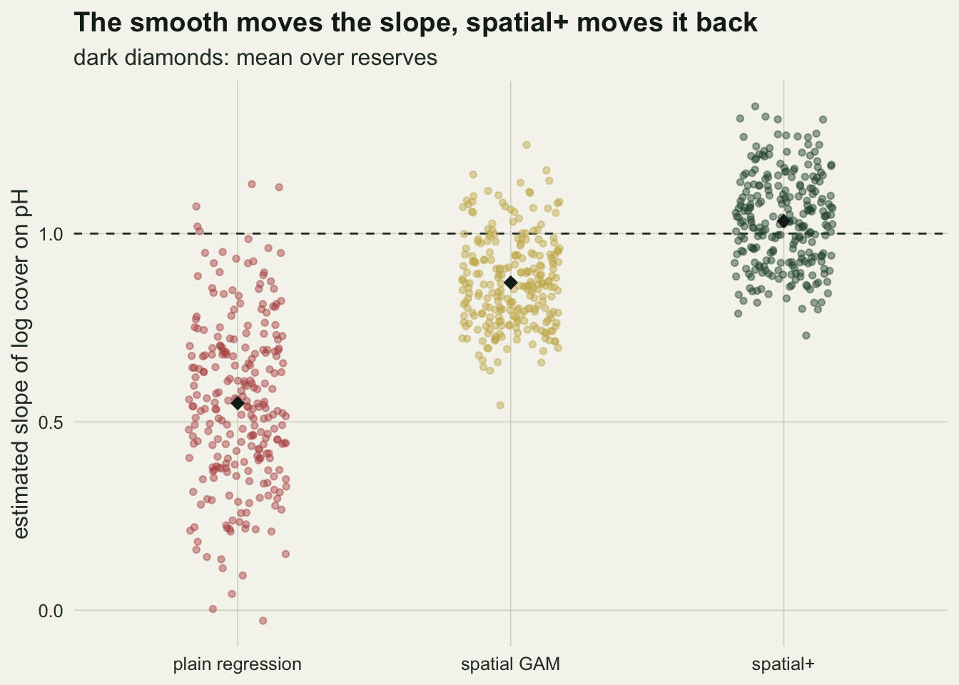
The direction of the bias is set by the sign of the confounding correlation, which was fixed at a negative value for the grazing story. A shorter run with the sign reversed shows the mirror image.
n_rep_flip <- 80
set.seed(9032)
tab_flip <- summarise_reps(t(replicate(n_rep_flip, one_rep(r = -r_conf))), "sign reversed")
tab_flip[, c("method", "mean_est", "sd_est", "coverage")]
method mean_est sd_est coverage
1 plain regression 1.411223 0.2239764 0.0875
2 spatial GAM 1.125879 0.1107209 0.7625
3 spatial+ 1.028504 0.1143650 0.9875flip_mcse_plus <- mcse_mean(tab_flip, 3)With the correlation at 0.6 and 80 reserves, the plain slope averages 1.411, the spatial GAM 1.126 and spatial+ 1.029. The plain and GAM biases flip sign with about the same size, so the attenuation in the title is a property of this grazing scenario: the spatial GAM is pulled toward the plain estimate, whichever side of the truth that lies on. Spatial+ stays above the truth in both runs (Monte Carlo standard error here 0.013), so the sign of its small bias is not set by the confounder.
Without a confounder the damage is to the interval
The same machinery with the correlation set to zero gives a reserve where the grazing legacy still varies smoothly in space but has nothing to do with bedrock. This is spatial autocorrelation in the residual and nothing more.
n_rep_clean <- 150
set.seed(9033)
tab_clean <- summarise_reps(t(replicate(n_rep_clean, one_rep(r = 0))), "no confounding")
mcse_cov_clean <- sqrt(0.95 * 0.05 / n_rep_clean)
se_ratio_ols <- at(tab_clean, 1, "sd_est") / at(tab_clean, 1, "mean_se")
width_ratio <- at(tab_clean, 3, "width") / at(tab_clean, 2, "width")
plus_cov_gap_z <- (0.95 - at(tab_clean, 3, "coverage")) / mcse_cov_clean
tab_clean[, c("method", "mean_est", "sd_est", "mean_se", "coverage")]
method mean_est sd_est mean_se coverage
1 plain regression 1.012291 0.2381970 0.07789699 0.4400000
2 spatial GAM 1.006592 0.1120583 0.10646391 0.9533333
3 spatial+ 1.046334 0.1267492 0.12396479 0.9200000Here the plain regression averages 1.012 with a Monte Carlo standard error of 0.019, so its point estimate is not the problem. Its standard error is: the estimates scatter 3.1 times as widely as the reported standard error claims, and its interval covers the truth 0.440 of the time. The spatial GAM averages 1.007 and covers 0.953; spatial+ averages 1.046 and covers 0.920, with an interval 1.16 times as wide as the GAM’s. The Monte Carlo standard error of a coverage near 0.95 at this replication is 0.018, so the spatial+ shortfall is 1.7 standard errors: suggestive, not established. With nothing confounded the spatial GAM is the better tool, and spatial+ buys nothing for its wider interval. The standard error problem on its own is the one that generalised least squares was built for.
cov_tab <- rbind(tab_conf, tab_clean)
cov_tab$scenario <- factor(cov_tab$scenario, levels = c("no confounding", "grazing confounded"))
cov_tab$mcse <- sqrt(cov_tab$coverage * (1 - cov_tab$coverage) / cov_tab$n_rep)
ggplot(cov_tab, aes(method, coverage, colour = method)) +
  geom_hline(yintercept = 0.95, colour = te_body, linetype = "dashed", linewidth = 0.5) +
  geom_errorbar(aes(ymin = pmax(0, coverage - 2 * mcse), ymax = pmin(1, coverage + 2 * mcse)),
                width = 0.2, linewidth = 0.5) +
  geom_point(size = 3) +
  facet_wrap(~ scenario) +
  scale_colour_manual(values = c(te_rust, te_gold, te_forest), guide = "none") +
  scale_y_continuous(limits = c(0, 1)) +
  labs(x = NULL, y = "interval coverage of the true slope",
       title = "Coverage with and without confounding",
       subtitle = "dashed line: the nominal 0.95") +
  theme_datasheet() +
  theme(axis.text.x = element_text(angle = 20, hjust = 1),
        strip.text = element_text(colour = te_ink, face = "bold"))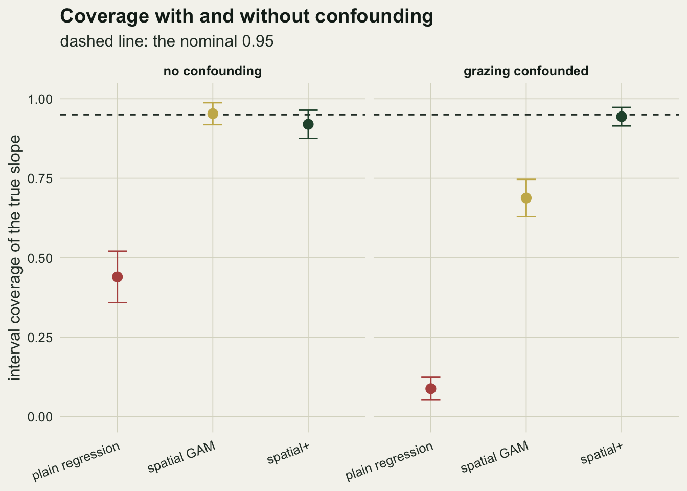
Spatial+ needs pH that is not spatial
Everything spatial+ knows about the slope comes from the residual of the first stage. If the plots differ in pH only because the bedrock differs, that residual is close to noise from the smoother, and there is nothing left to estimate from. The last run holds the confounding at its design value and varies the plot-level standard deviation of pH.
sd_grid <- c(0.1, 0.25, 0.5, 1)
n_rep_sweep <- 80
set.seed(9034)
sweep <- do.call(rbind, lapply(sd_grid, function(s) {
  if (s == sd_local) {
    tb <- tab_conf
  } else {
    tb <- summarise_reps(t(replicate(n_rep_sweep, one_rep(sd_x = s))), "sweep")
  }
  tb$sd_x <- s; tb$share <- s^2 / (1 + s^2); tb
}))
sweep$mcse <- sweep$sd_est / sqrt(sweep$n_rep)
sw <- function(s, m, col) sweep[sweep$sd_x == s & sweep$method == method_lev[m], col]
sweep[, c("share", "method", "mean_est", "coverage", "width")]
share method mean_est coverage width
1 0.00990099 plain regression 0.4269955 0.0875 0.3283274
2 0.00990099 spatial GAM 0.5005804 0.2875 0.7535812
3 0.00990099 spatial+ 1.1011468 0.9875 2.3685990
4 0.05882353 plain regression 0.4803383 0.1125 0.3087135
5 0.05882353 spatial GAM 0.6489517 0.3500 0.6019679
6 0.05882353 spatial+ 1.0228356 0.9750 0.9820021
7 0.20000000 plain regression 0.5495525 0.0880 0.2894694
8 0.20000000 spatial GAM 0.8699727 0.6880 0.4114853
9 0.20000000 spatial+ 1.0332871 0.9440 0.4876491
10 0.50000000 plain regression 0.7344713 0.0875 0.2195362
11 0.50000000 spatial GAM 0.9708301 0.9250 0.2291883
12 0.50000000 spatial+ 1.0304616 0.9125 0.2429956plus_bias_all <- c(at(tab_flip, 3, "mean_est"), at(tab_clean, 3, "mean_est"),
sweep$mean_est[sweep$method == method_lev[3]]) - beta_set
plus_mcse_all <- c(mcse_mean(tab_flip, 3), mcse_mean(tab_clean, 3),
sweep$mcse[sweep$method == method_lev[3]])
plus_bias_z_all <- plus_bias_all / plus_mcse_all
mcse_cov_sweep <- sqrt(0.95 * 0.05 / n_rep_sweep)At the smallest plot-level variation, 1 per cent of the variance in pH, the first-stage residual keeps 1 per cent of it on average. Spatial+ still centres near the truth, at 1.10 with a Monte Carlo standard error of 0.06, and its interval still covers (0.988). It covers because it is 2.37 units wide on a true slope of 1: centred where it is, the average interval runs from -0.08 to 2.29, which takes in both no effect and twice the real one. The spatial GAM there averages 0.50 with an interval 0.75 wide, so it is narrower and wrong, and covers 0.287 of the time.
So the failure of spatial+ when the covariate is almost purely spatial is not bias but emptiness, and it announces itself through the interval width, which is the honest way to fail. The spatial GAM fails silently in the same corner. At 6 per cent plot-level variation the spatial+ interval is 0.98 wide; at 50 per cent it is 0.24, and the spatial GAM has caught up to 0.971, because with that much non-spatial pH the smooth no longer has much to compete for. The plain regression is still at 0.734. Coverages in this sweep carry a Monte Carlo standard error of about 0.024 near 0.95.
p_bias <- ggplot(sweep, aes(share, mean_est, colour = method)) +
  geom_hline(yintercept = beta_set, colour = te_body, linetype = "dashed", linewidth = 0.5) +
  geom_errorbar(aes(ymin = mean_est - 2 * mcse, ymax = mean_est + 2 * mcse), width = 0.02, linewidth = 0.4) +
  geom_line(linewidth = 0.9) + geom_point(size = 2.2) +
  scale_colour_manual(values = c(te_rust, te_gold, te_forest), name = NULL) +
  labs(x = "plot-level share of pH variance", y = "mean slope estimate",
       title = "Bias", subtitle = "dashed line: the true slope") +
  theme_datasheet()
p_width <- ggplot(sweep, aes(share, width, colour = method)) +
  geom_line(linewidth = 0.9) + geom_point(size = 2.2) +
  scale_y_log10(breaks = c(0.25, 0.5, 1, 2)) +
  scale_colour_manual(values = c(te_rust, te_gold, te_forest), guide = "none") +
  labs(x = "plot-level share of pH variance", y = "mean 95 per cent interval width",
       title = "Price", subtitle = "log scale, same colours") +
  theme_datasheet()
p_bias + p_width + plot_layout(guides = "collect") +
  plot_annotation(theme = theme_datasheet()) & theme(legend.position = "bottom")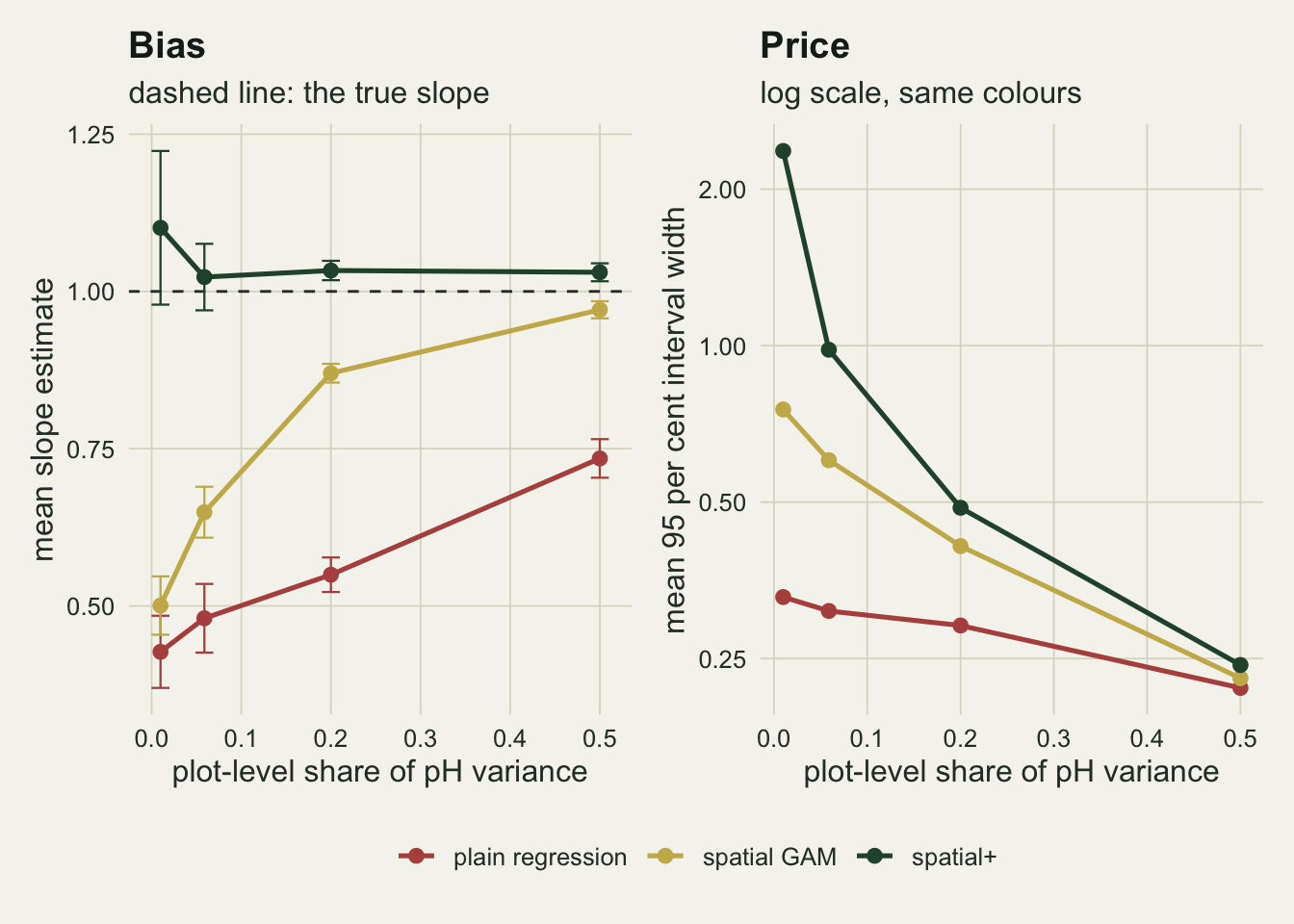
Where the small upward bias of spatial+ comes from
Spatial+ averaged above the truth in all 6 simulated settings above, by between 0.023 and 0.101, and in 4 of them by more than two Monte Carlo standard errors. That includes both signs of the confounding and the run with no confounding at all, so the confounder is not what sets its sign. The smoothing is.
Once REML has chosen the smoothing parameter, the second-stage fit is penalised least squares, and the spatial+ slope is a weighted sum of the cover values. The weights come from the model matrix and the scaled covariance matrix Vp / sig2 that gam() returns. Cover is the slope times pH, plus the grazing legacy, plus noise, and pH is the first-stage smooth plus its residual. Because the residual column carries no penalty, the weights applied to it return exactly one, so the slope times the residual contributes exactly the true slope. The bias is then what the weights pick up from the other ingredients: the slope times the smooth part of pH, the grazing legacy, and noise, whose contribution has mean zero apart from the small dependence of the smoothing parameter on the noise. The chunk computes each piece on the confounded design, for three basis dimensions of the first-stage smooth of pH, with the second stage held at the design basis of 50.
g_ph_k30  <- gam(ph ~ s(lon, lat, k = 30), data = res1, method = "REML", fit = FALSE)
g_ph_k100 <- gam(ph ~ s(lon, lat, k = 100), data = res1, method = "REML", fit = FALSE)
split_plus <- function(g_x, d) {
  stage1 <- refit(g_x, d$ph)
  ph_r <- residuals(stage1); ph_f <- fitted(stage1)
  stage2 <- refit(g_cover, d$cover, ph_r)
  x_mat <- g_cover$X; x_mat[, 2] <- ph_r
  w_slope <- ((stage2$Vp / stage2$sig2) %*% t(x_mat))[2, ]
  noise <- d$cover - beta_set * d$ph - d$grazing
  c(est = unname(coef(stage2)[2]),
    smooth_part = sum(w_slope * beta_set * ph_f),
    grazing_part = sum(w_slope * d$grazing),
    noise_part = sum(w_slope * noise),
    check = max(abs(sum(w_slope * d$cover) - coef(stage2)[2]), abs(sum(w_slope * ph_r) - 1)),
    cor_fit_resid = cor(ph_r, ph_f))
}
n_rep_split <- 40   # fixed before any result was seen
set.seed(9035)
reps_split <- replicate(n_rep_split, {
  d <- draw_reserve()
  rbind(k30 = split_plus(g_ph_k30, d), k50 = split_plus(g_ph, d), k100 = split_plus(g_ph_k100, d))
})
systematic <- reps_split[, "smooth_part", ] + reps_split[, "grazing_part", ]
split_tab <- data.frame(k_x = c(30, k_sp, 100),
                        mean_est = apply(reps_split[, "est", ], 1, mean),
                        mcse_est = apply(reps_split[, "est", ], 1, sd) / sqrt(n_rep_split),
                        smooth_part = apply(reps_split[, "smooth_part", ], 1, mean),
                        grazing_part = apply(reps_split[, "grazing_part", ], 1, mean),
                        noise_part = apply(reps_split[, "noise_part", ], 1, mean),
                        mcse_noise = apply(reps_split[, "noise_part", ], 1, sd) / sqrt(n_rep_split),
                        systematic = rowMeans(systematic),
                        mcse_sys = apply(systematic, 1, sd) / sqrt(n_rep_split),
                        cor_fit_resid = apply(reps_split[, "cor_fit_resid", ], 1, mean))
split_check <- max(reps_split[, "check", ])
sp_row <- function(k, col) split_tab[split_tab$k_x == k, col]
round(split_tab, 4)
k_x mean_est mcse_est smooth_part grazing_part noise_part mcse_noise
k30 30 0.9808 0.0181 0.0322 -0.0294 -0.0220 0.0182
k50 50 1.0068 0.0197 0.0566 -0.0287 -0.0211 0.0197
k100 100 1.0388 0.0211 0.0922 -0.0309 -0.0225 0.0206
systematic mcse_sys cor_fit_resid
k30 0.0029 0.0016 0.0502
k50 0.0280 0.0018 0.0694
k100 0.0613 0.0029 0.0894The weighted-sum split reproduces the fitted slope and the unit weight on the residual to within 2.4e-15. With the same basis in both stages, the first-stage residual still correlates at 0.069 with the fitted smooth part of pH, averaged over 40 reserves: a penalised smooth does not take out everything smooth. The second-stage smooth does not absorb all of the slope times that smooth part either, and what it leaves loads onto the residual column. That term averages 0.057. The grazing legacy leaks the other way, -0.029, and the noise term averages -0.021 with a Monte Carlo standard error of 0.020. The systematic sum, 0.028 with a Monte Carlo standard error of 0.002, is the bias apart from that noise term. It is measured far more precisely than the mean estimate itself (1.007, standard error 0.020), because it leaves out the noise. The smooth-part term is the true slope times a weighted sum of the smooth part of pH, so it vanishes when the true slope is zero (the grazing term does not contain the slope, so it would not vanish with it), and the grazing legacy enters it only through the chosen smoothing parameter. That is why the upward bias turned up with both signs of the confounding and without any.
The basis of the first stage moves it. With k = 30 for the smooth of pH the smooth-part term drops to 0.032 and the systematic bias to 0.003, 1.8 standard errors from zero; with k = 100 they rise to 0.092 and 0.061 (standard error 0.003). The grazing term hardly changes, -0.029 against -0.031, so at the smoothness of these fields a thirty-dimensional first stage still takes out the part of pH that the grazing legacy is correlated with. A first stage richer than the second puts part of the smooth of pH outside what the second-stage smooth can represent, and the slope times that part is left over for the residual column to take.
What to report
Report the spatial GAM slope and the spatial+ slope side by side, with their intervals. They answer the same question under different assumptions about where the identifying variation comes from, and a large distance between them is the most direct evidence a reader gets that the smooth and the covariate were competing. On the worked reserve that distance was 0.10; across the confounded simulation it averaged 0.16. Part of any such distance is the upward smoothing bias of spatial+ itself: without confounding the spatial GAM is centred on the truth and the gap still averaged 0.04, so a gap of that size says nothing about competition.
Report the first stage. The effective degrees of freedom of the smooth of the covariate on the coordinates, and the share of the covariate’s variance left in its residual, tell a reader how much information the spatial+ slope stands on. A residual share of a few per cent means the estimate rests on a small part of the covariate’s variance, and the interval will say so; a reader should not need to rerun the model to find that out.
Report the basis dimension of both smooths, and keep the basis of the covariate smooth no larger than the basis of the response smooth. In the measurement above a first-stage basis twice the size of the second multiplied the systematic bias by 2.2, and a first-stage basis of 30 brought it down from 0.028 to 0.003. Going smaller has its own risk that this design did not test: a first stage too coarse to represent the confounded part of the covariate leaves that part in the residual, where it brings the confounding back.
Do not describe the spatial+ slope as a causal effect of pH. It is protected against a confounder that varies smoothly in space at the scale the basis can represent. A driver that varies from plot to plot together with pH gets through untouched.
Honest limits
The confounder in these simulations is exactly as smooth as the spatial part of pH, and both are well inside what a fifty-dimensional thin plate basis represents on a ten kilometre square. Paciorek 2010 shows how much the relative scales of covariate and confounder decide the bias of spatial regression estimators, and only one pair of scales was run here. A confounder that varies at a finer scale than the basis can capture was not simulated; neither the spatial GAM nor spatial+ would see it.
The plot-level variation in pH was drawn independent of everything else, which is the assumption spatial+ lives on. A boulder that raises pH and also shades the herb would put a local confounder into exactly the variation the method uses, and no amount of spatial smoothing removes it.
The split of the spatial+ bias holds the smoothing parameter at the value REML chose in each replicate, as Vp does; it describes the fitted estimator, not a theory of how the bias shrinks with sample size. The basis comparison used 40 reserves, three first-stage bases and one second-stage basis, on the confounded design only. The second-stage standard error also treats the first-stage residual as known data, and the coverage without confounding fell a little short of nominal; with 150 replicates that shortfall cannot be separated from simulation noise.
Everything here is one layout of 300 plots, a Gaussian response, one covariate and one correlation length. The replication runs from 80 to 250 reserves, which keeps the whole post fast enough to knit but leaves coverage in the sweep with standard errors of a couple of percentage points. Spatial+ extends to generalised responses and several covariates in the original paper; none of that was run here.
Restricted spatial regression, the remedy named in the diagnostic post, was not compared. For a Gaussian linear model it returns the plain regression slope by construction, which in the confounded scenario here is the most biased of the three estimates.
References
Dupont E, Wood SN, Augustin NH 2022 Biometrics 78(4):1279-1290 (10.1111/biom.13656)
Hodges JS, Reich BJ 2010 The American Statistician 64(4):325-334 (10.1198/tast.2010.10052)
Paciorek CJ 2010 Statistical Science 25(1):107-125 (10.1214/10-STS326)
Wood SN 2017 Generalized Additive Models: An Introduction with R, 2nd edition (ISBN 978-1-4987-2833-1)