Moran eigenvector spatial filtering

Turn a spatial weights matrix into orthogonal map patterns, add them to a Poisson GLM to remove residual autocorrelation, and see where filtering falls short.

Corrected 14 October 2026: the take-away and the end of the simulation section stated as a general property of filtering that it lowers the false-positive rate but leaves it well above nominal, which the post measured for one unmeasured field only; they now tie that result to the simulation. The residual autocorrelation of the filtered model is now called no longer significant by the raw-data test that drives the stopping rule, rather than no longer significant outright.

Corrected 1 October 2026: many eigenvector maps on this grid share an eigenvalue, and the orientation that eigen() returns for such tied maps is arbitrary and can differ between computers, so selecting single maps made the results depend on the machine; tied sets of maps now enter the model whole, which gives the same answer for any orientation, a higher false-positive rate under filtering than the post reported and a more guarded verdict. The post also no longer cites Diniz-Filho et al. for a red-herring warning that their paper argues against, nor says that autocorrelation can flip the sign of a relationship, and it now says that the covariate’s smooth pattern, not only the field, is held fixed across replicates.

Corrected 27 September 2026: the post called the drop in false positives under filtering a roughly fivefold reduction that still left the rate more than triple the nominal five per cent, which the printed rates did not support; both ratios are now computed from the simulation.

The SAR and CAR models are built for Gaussian responses. Ecological areal data are often counts or presences, where you would rather stay inside a Poisson or binomial generalised linear model. Fitting a full autoregressive likelihood for those families is awkward. Moran eigenvector spatial filtering offers a lighter alternative: it distils the neighbourhood structure into a handful of orthogonal map patterns, then drops them into an ordinary GLM as extra covariates. The spatial autocorrelation is soaked up by the patterns, and everything else about the model stays familiar.

This tutorial builds the eigenvector maps by hand, confirms that each one’s Moran’s I equals a scaled eigenvalue, and uses forward selection to clean the residual autocorrelation out of a Poisson regression. It also does something many treatments avoid: it measures, across many simulated datasets, how well filtering actually controls the false positives that spatial autocorrelation causes. The answer is less reassuring than the clean residuals suggest.

Map patterns from a weights matrix

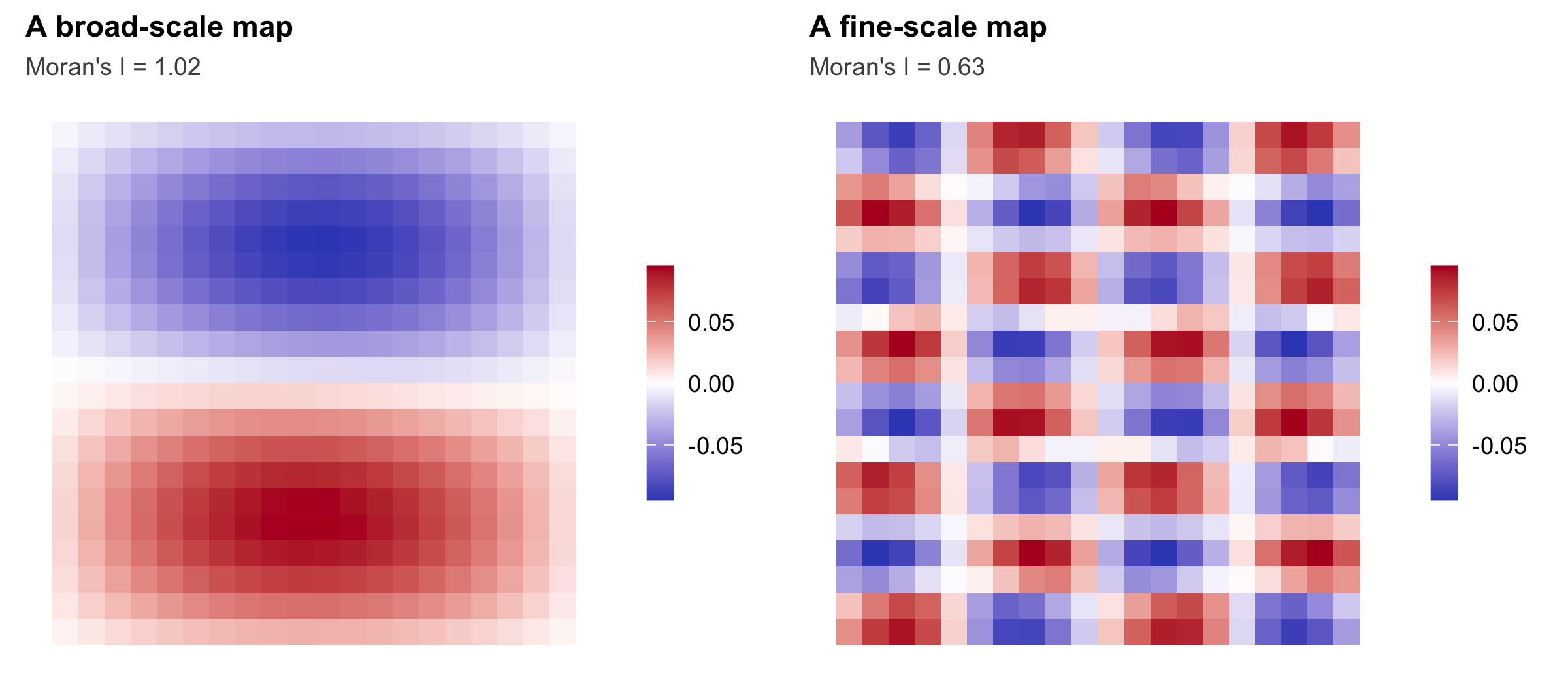
Take the binary adjacency matrix A, centre it on both sides with C = I - 11'/n, and find the eigenvectors of C A C. Those eigenvectors, the Moran eigenvector maps (MEM), are mutually orthogonal spatial patterns. The one with the largest eigenvalue is the broadest gradient across the map; later ones describe progressively finer structure; and eigenvectors with negative eigenvalues encode negative autocorrelation, the checkerboards. The tidy fact that makes them useful is that the Moran’s I of eigenvector k is exactly (n / sum(A)) times its eigenvalue.

library(ggplot2)
library(grid)
knitr::opts_chunk$set(echo = TRUE, message = FALSE, warning = FALSE,
                      dev = "png", dev.args = list(bg = "#f5f4ee"),
                      dpi = 150, fig.width = 8, fig.height = 3.5)
theme_te <- function() {
  theme_minimal(base_size = 11) +
    theme(plot.background = element_rect(fill = "#f5f4ee", colour = NA),
          panel.background = element_rect(fill = "#f5f4ee", colour = NA),
          panel.grid = element_blank(),
          plot.title = element_text(face = "bold", size = 11),
          plot.subtitle = element_text(size = 9, colour = "grey30"),
          axis.text = element_blank(), axis.ticks = element_blank(),
          legend.key.width = unit(0.35, "cm"))
}
memmap <- function(coords, value, title, subtitle = NULL) {
  df <- data.frame(col = coords$col, row = coords$row, v = value)
  ggplot(df, aes(col, row, fill = v)) + geom_tile() + coord_equal() +
    scale_fill_gradient2(low = "#3b4cc0", mid = "white", high = "#b40426",
                         midpoint = 0) +
    labs(title = title, subtitle = subtitle, x = NULL, y = NULL, fill = NULL) +
    theme_te()
}
two_panel <- function(g1, g2) {
  grid.newpage(); pushViewport(viewport(layout = grid.layout(1, 2)))
  print(g1, vp = viewport(layout.pos.row = 1, layout.pos.col = 1))
  print(g2, vp = viewport(layout.pos.row = 1, layout.pos.col = 2))
}
moran_test <- function(z, W) {
  n <- length(z); z <- z - mean(z)
  S0 <- sum(W); S1 <- 0.5 * sum((W + t(W))^2)
  S2 <- sum((rowSums(W) + colSums(W))^2)
  I  <- (n / S0) * as.numeric(t(z) %*% W %*% z) / sum(z^2)
  EI <- -1 / (n - 1); b2 <- n * sum(z^4) / (sum(z^2)^2)
  VI <- (n * ((n^2 - 3 * n + 3) * S1 - n * S2 + 3 * S0^2)
         - b2 * ((n^2 - n) * S1 - 2 * n * S2 + 6 * S0^2)) /
        ((n - 1) * (n - 2) * (n - 3) * S0^2) - EI^2
  list(I = I, p = pnorm((I - EI) / sqrt(VI), lower.tail = FALSE))
}

side <- 20; n <- side * side
coords <- expand.grid(col = 1:side, row = 1:side)
A <- matrix(0, n, n)
idx <- function(r, c) (c - 1) * side + r
for (r in 1:side) for (c in 1:side) {
  i <- idx(r, c)
  if (r > 1)    A[i, idx(r - 1, c)] <- 1
  if (r < side) A[i, idx(r + 1, c)] <- 1
  if (c > 1)    A[i, idx(r, c - 1)] <- 1
  if (c < side) A[i, idx(r, c + 1)] <- 1
}
one <- rep(1, n); Cn <- diag(n) - outer(one, one) / n
eg  <- eigen(Cn %*% A %*% Cn, symmetric = TRUE)
keep <- abs(eg$values) > 1e-8
E <- eg$vectors[, keep]                       # the eigenvector maps
moranE <- (n / sum(A)) * eg$values[keep]      # Moran's I of each map
grp <- cumsum(c(TRUE, abs(diff(moranE)) > 1e-8))  # maps with tied eigenvalues share a group
broad <- which(moranE > 0)[order(-moranE[moranE > 0])]  # broad patterns first
mem_npos <- length(broad)

A quick check confirms the eigenvalue identity: the analytic Moran’s I of a map agrees with a direct computation.

k <- broad[1]
c(from_eigenvalue = moranE[k], from_moran_test = moran_test(E[, k], A)$I)

from_eigenvalue from_moran_test 
        1.02337         1.02337 

The two agree to machine precision. Double centring leaves 379 maps with a non-zero eigenvalue, fewer than the n - 1 you might expect, because a regular square grid has a block of exactly zero eigenvalues. Of those maps, 189 carry positive autocorrelation.

Two Moran eigenvector maps from the same weights matrix: a broad-scale gradient across the grid and a fine-scale alternating pattern, each labelled with the Moran’s I implied by its eigenvalue.

A spatial red herring

Here is the trap that filtering is meant to defuse. We simulate a spatially structured covariate that has no real effect on the response, alongside an unmeasured smooth field that does drive the counts. Because both the covariate and the response carry spatial structure, a naive analysis is prone to see a relationship that is not there.

set.seed(4233)
x   <- as.numeric(scale(1.1 * sin(pi * coords$col / 11) -
                        0.9 * cos(pi * coords$row / 12) + rnorm(n, 0, 0.5)))
fsp <- as.numeric(scale(1.2 * sin(pi * coords$col / 8 + 0.6) +
                        1.0 * cos(pi * coords$row / 7 - 0.4)))  # unmeasured field
b0 <- 1.4; b1_true <- 0
set.seed(20)
y <- rpois(n, exp(b0 + b1_true * x + 0.85 * fsp))
c(mean = mean(y), zeros = sum(y == 0), max = max(y))

   mean   zeros     max 
 5.7875 30.0000 27.0000 

Fit the count model that ignores space and inspect both the covariate and the residual autocorrelation.

g0 <- glm(y ~ x, family = poisson)
s0 <- summary(g0)$coefficients
mem_base_b1    <- s0["x", "Estimate"]
mem_base_se    <- s0["x", "Std. Error"]
mem_base_z     <- s0["x", "z value"]
mem_base_p     <- s0["x", "Pr(>|z|)"]
mem_base_moran <- moran_test(residuals(g0, type = "pearson"), A)$I
round(c(b1 = mem_base_b1, se = mem_base_se, z = mem_base_z,
        p = mem_base_p, resid_moran = mem_base_moran), 4)

         b1          se           z           p resid_moran 
    -0.0738      0.0209     -3.5326      0.0004      0.7178 

The covariate looks convincingly significant, with a z of -3.53 and a p-value of \(4.1 \times 10^{-4}\), yet its true effect is zero. The Pearson residuals carry a Moran’s I of 0.72, a blazing signal of leftover spatial structure. Diniz-Filho et al. (2003) accept that spatial autocorrelation can inflate Type I errors, while arguing that it does not necessarily bias the estimates; here it manufactures false confidence in a covariate with no effect at all.

Filtering it out

Forward selection adds eigenvector maps step by step, each time choosing the map most correlated with the current residuals, and stops once the residual autocorrelation is no longer significant. We restrict the candidates to the broad-scale maps, where a smooth field lives. A square grid needs one extra rule. Many of its maps come in pairs, and a few in larger sets, that share exactly the same eigenvalue, and any rotation of such a tied set is an equally valid set of maps; which rotation eigen() returns is arbitrary and can differ from one computer to the next. Picking single maps out of a tied set would make the result depend on that accident, so each tied set competes as one candidate, scored by the share of the residual variation its maps explain together (for a single map, its squared correlation), and enters the model whole.

cand <- broad[1:80]; sel <- integer(0); r <- resid(lm(y ~ x))
for (s in 1:25) {
  if (moran_test(r, A)$p > 0.05) break
  left <- setdiff(grp[cand], grp[sel])            # tied sets not yet in the model
  sc <- sapply(left, function(g) sum(crossprod(E[, grp == g, drop = FALSE], r)^2))
  sel <- c(sel, which(grp == left[which.max(sc)])) # add the whole tied set
  r <- resid(lm(y ~ x + E[, sel]))
}
gm <- glm(y ~ x + E[, sel], family = poisson)
sm <- summary(gm)$coefficients
mem_nsel      <- length(sel)
mem_filt_b1   <- sm["x", "Estimate"]
mem_filt_se   <- sm["x", "Std. Error"]
mem_filt_z    <- sm["x", "z value"]
mem_filt_p    <- sm["x", "Pr(>|z|)"]
mem_filt_moran <- moran_test(residuals(gm, type = "pearson"), A)$I
round(c(n_maps = mem_nsel, b1 = mem_filt_b1, se = mem_filt_se,
        z = mem_filt_z, p = mem_filt_p, resid_moran = mem_filt_moran), 4)

     n_maps          b1          se           z           p resid_moran 
    23.0000      0.0017      0.0447      0.0370      0.9705      0.0342 

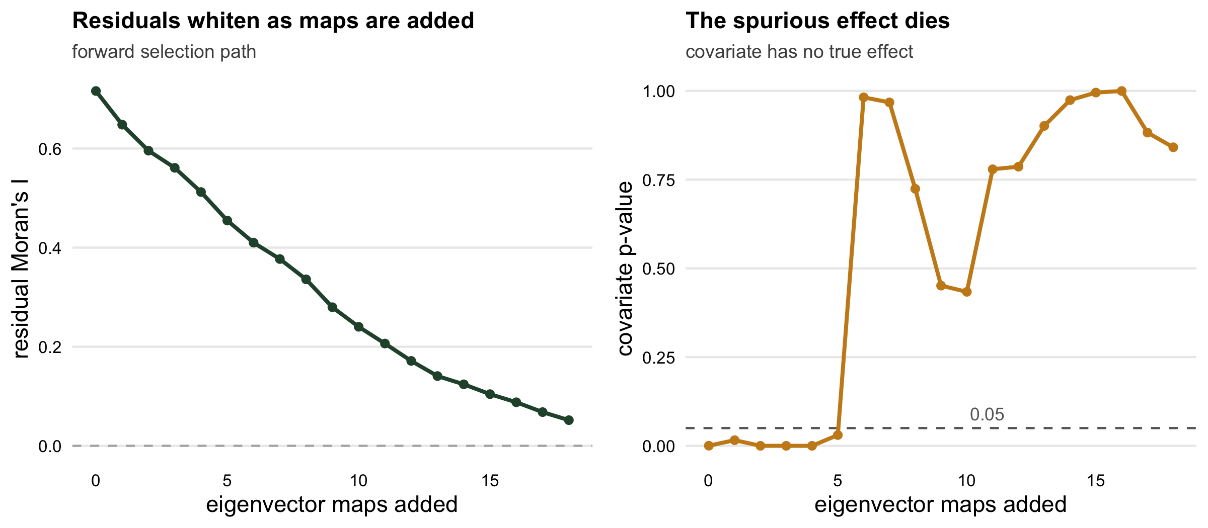
Adding 23 maps pulls the residual Moran’s I down from 0.72 to 0.034, no longer significant by the raw-data test that drives the stopping rule, and the spurious effect evaporates: the covariate’s p-value climbs from \(4.1 \times 10^{-4}\) to 0.97. The GLM machinery never changed. We simply gave it enough spatial patterns to explain the clustering that the covariate was otherwise blamed for.

The stopping rule judges the residuals of lm(y ~ x + maps) against EI <- -1 / (n - 1), the null of raw data. Residuals of a model that already holds many broad maps have a lower null mean, so this rule tends to stop earlier than a test on the residual null would; with Poisson counts either test is an approximation. The comparison is measured in Moran’s I on residuals, where the residual rule changes the number of maps kept but not the false-positive rate of a confounded covariate.

Forward selection of eigenvector maps, one map or tied set of maps at a time. Left: the residual Moran’s I falls towards zero as maps enter the model. Right: the covariate’s p-value climbs past the 0.05 line, falls back below it for two steps and then settles well above it, so the effect that looked significant was the spatial pattern all along.

Does filtering really fix the inference?

Removing autocorrelation from one dataset is reassuring but not proof. The sterner test is to repeat the whole procedure on many datasets where the covariate genuinely has no effect, and count how often each method wrongly declares it significant. We compare the naive Poisson GLM with adaptive filtering, selecting maps afresh for every dataset.

select_mem <- function(y, x, cand, maxK = 25) {
  sel <- integer(0); r <- resid(lm(y ~ x))
  for (s in 1:maxK) {
    if (moran_test(r, A)$p > 0.05) break
    left <- setdiff(grp[cand], grp[sel])
    sc <- sapply(left, function(g) sum(crossprod(E[, grp == g, drop = FALSE], r)^2))
    sel <- c(sel, which(grp == left[which.max(sc)])); r <- resid(lm(y ~ x + E[, sel]))
  }
  sel
}
mkx <- function(seed) { set.seed(seed)
  as.numeric(scale(1.1 * sin(pi * coords$col / 11) -
                   0.9 * cos(pi * coords$row / 12) + rnorm(n, 0, 0.5))) }
fb <- fsp                       # one unmeasured field, held fixed across replicates
B <- 300; naive <- adapt <- logical(B); nsel <- integer(B)
for (b in 1:B) {
  xb <- mkx(10000 + b); set.seed(20000 + b)
  yb <- rpois(n, exp(b0 + 0 * xb + 0.85 * fb))
  naive[b] <- summary(glm(yb ~ xb, family = poisson))$coefficients["xb", "Pr(>|z|)"] < 0.05
  se <- select_mem(yb, xb, broad[1:80]); nsel[b] <- length(se)
  adapt[b] <- summary(glm(yb ~ xb + E[, se], family = poisson))$coefficients["xb", "Pr(>|z|)"] < 0.05
}
mem_mc_naive <- mean(naive); mem_mc_adapt <- mean(adapt); mem_mc_medk <- median(nsel)
round(c(naive = mem_mc_naive, filtered = mem_mc_adapt, median_maps = mem_mc_medk), 3)

      naive    filtered median_maps 
      0.903       0.290      24.000 

The naive GLM is a disaster: it flags the null covariate as significant 90 per cent of the time, not the nominal five. Adaptive filtering, using a median of 24 maps, cuts that to 29 per cent. That is a real improvement, a reduction by a factor of about 3, but it is honestly still about 5.8 times the nominal rate. Both rates are conditional on this one unmeasured field and on the smooth pattern of the covariate, both held fixed across the 300 replicates while only the covariate’s independent noise and the counts are redrawn; another confounding pattern would give different numbers. Here filtering helps; it is far from a cure.

This matches what the literature found the hard way. Bini et al. (2009) compared spatial and non-spatial regression across dozens of real datasets and concluded that the shifts in coefficients are largely idiosyncratic, with no reliable rule for when a spatial method will behave. In this simulation eigenvector filtering reduced the red herring without eliminating it, and the number of maps you keep is a genuine tuning choice that trades false positives against power.

What to carry forward

Moran eigenvector filtering is the pragmatic choice when your response is a count or a presence and a full SAR or CAR likelihood is more than you want to fit. It converts the neighbourhood into orthogonal map patterns, and a modest selection of them, added as covariates, strips most of the spatial autocorrelation out of the residuals. That whitening is real and worth having.

Keep two things in view. The maps are patterns, not mechanisms; they describe where the response clusters, not why, so they support honest inference rather than causal claims. And the control they buy depends on the setting: in the simulation above, false-positive rates fell but stayed well above nominal for its one unmeasured field, and the choice of how many maps to keep matters. When the covariate you care about is itself spatially smooth, those same maps can start absorbing its signal, which is the confounding problem that checking a spatial regression confronts directly.

References

Bini LM, Diniz-Filho JAF, Rangel TFLVB, Akre TSB, et al. 2009 Ecography 32(2):193-204 (10.1111/j.1600-0587.2009.05717.x)

Diniz-Filho JAF, Bini LM & Hawkins BA 2003 Global Ecology and Biogeography 12(1):53-64 (10.1046/j.1466-822X.2003.00322.x)

Dray S, Legendre P & Peres-Neto PR 2006 Ecological Modelling 196(3-4):483-493 (10.1016/j.ecolmodel.2006.02.015)

Griffith DA & Peres-Neto PR 2006 Ecology 87(10):2603-2613 (10.1890/0012-9658(2006)87[2603:SMIETF]2.0.CO;2)

Related tutorials

• Join counts for presence-absence maps test whether presences and absences cluster on a map, before any model is fitted.
• Conditional autoregressive (CAR) models build autoregressive dependence for Gaussian responses from local conditionals.
• Checking a spatial regression tests which spatial model fits and exposes spatial confounding.
• Moran’s I on residuals: moran.test or lm.morantest tests residuals against their own null rather than that of raw data, and measures what that does to this stopping rule.

Reproducibility

• Code last run: 2026-10-15
• R version 4.5.3 (2026-03-11), aarch64-apple-darwin20
• Packages: ggplot2 4.0.3