Checking a spatial regression

Diagnose an areal spatial model with residual Moran’s I and Lagrange multiplier tests, compare SAR, CAR and filtering, and confront spatial confounding.

You have fitted a spatial model, a spatial lag or error model, a conditional autoregressive model, or a Moran eigenvector filter. Three questions decide whether to trust it. Did the model actually remove the spatial autocorrelation it was meant to? Which specification do the data prefer? And, the question most tutorials duck, is the covariate effect you care about still identified once space is in the model? This closing tutorial answers all three in base R, and the third answer is a genuine caution rather than a reassurance.

Setting up

side <- 20; n <- side * side
coords <- expand.grid(col = 1:side, row = 1:side)
A <- matrix(0, n, n)
idx <- function(r, c) (c - 1) * side + r
for (r in 1:side) for (c in 1:side) {
  i <- idx(r, c)
  if (r > 1)    A[i, idx(r - 1, c)] <- 1
  if (r < side) A[i, idx(r + 1, c)] <- 1
  if (c > 1)    A[i, idx(r, c - 1)] <- 1
  if (c < side) A[i, idx(r, c + 1)] <- 1
}
deg <- rowSums(A); D <- diag(deg); W <- A / deg
ev <- eigen(diag(1 / sqrt(deg)) %*% A %*% diag(1 / sqrt(deg)), symmetric = TRUE)$values
rho_lo <- 1 / min(ev); rho_hi <- 1 / max(ev)
set.seed(4234)
x  <- as.numeric(scale(0.8 * sin(pi * coords$col / 7) +
                       0.6 * scale(coords$row)[, 1] + rnorm(n, 0, 0.6)))
X  <- cbind(1, x); b0 <- 0.6; b1 <- 0.7; sig <- 0.5

Check one: is the autocorrelation gone?

The workhorse diagnostic is Moran’s I on the residuals. Ordinary residuals from a well-specified spatial model should look spatially random. For a lag model the relevant residuals are the filtered innovations (I - rho W)y - X beta; for an error or CAR model they are the whitened innovations. In every earlier tutorial the pattern was the same: the naive model left a large residual Moran’s I, and the spatial model drove it towards zero. That single number, computed on the innovations rather than the raw response, is the first thing to report and the first thing a reviewer will ask for.

Check two: lag or error?

Residual Moran’s I tells you that autocorrelation is present, not which model to use. The Lagrange multiplier tests of Anselin et al. (1996) fill that gap. Both start from ordinary least squares residuals and ask whether adding a lag term, or an error term, would significantly improve the fit. We implement both by hand.

M  <- diag(n) - X %*% solve(crossprod(X)) %*% t(X)          # OLS annihilator
Tw <- sum(diag(crossprod(W))) + sum(diag(W %*% W))          # a weights constant
lm_tests <- function(y) {
  o <- lm(y ~ x); e <- resid(o); s2 <- sum(e^2) / n
  Wy <- as.numeric(W %*% y); We <- as.numeric(W %*% e)
  fit <- as.numeric(X %*% coef(o)); WXb <- as.numeric(W %*% fit)
  LMerr <- (sum(e * We) / s2)^2 / Tw
  Draj  <- as.numeric(t(WXb) %*% M %*% WXb) / s2 + Tw
  LMlag <- (sum(e * Wy) / s2)^2 / Draj
  c(LMerr = LMerr, LMlag = LMlag)
}

To see the tests discriminate, we simulate one dataset from a lag process and one from an error process, then run both tests on each.

set.seed(51); y_lag <- as.numeric(solve(diag(n) - 0.6 * W) %*% (X %*% c(b0, b1) + rnorm(n, 0, sig)))
set.seed(52); y_err <- as.numeric(X %*% c(b0, b1) + solve(diag(n) - 0.6 * W) %*% rnorm(n, 0, sig))
hl <- lm_tests(y_lag); he <- lm_tests(y_err)
chk_lmerr_lag <- hl["LMerr"]; chk_lmlag_lag <- hl["LMlag"]
chk_lmerr_err <- he["LMerr"]; chk_lmlag_err <- he["LMlag"]
rbind(`lag data` = round(hl, 1), `error data` = round(he, 1))

           LMerr LMlag
lag data    47.6 201.0
error data  90.4  45.8

The tests point the right way each time. On lag-generated data the lag statistic, 201, dwarfs the error statistic, 48. On error-generated data the ordering reverses, with the error statistic 90 above the lag statistic 46. Both are referred to a chi-squared distribution on one degree of freedom, and both by-hand values match spdep’s lm.LMtests to numerical precision. When the two statistics disagree in direction, follow the larger one; when they both fire, the adjusted forms in the same reference help decide.

Check three: which model fits best?

Tests are local; a global comparison rounds them out. We fit all five candidates to the lag-generated data and rank them by AIC alongside the residual autocorrelation each leaves behind. The spatial fits reuse the by-hand likelihoods from the earlier tutorials.

y <- y_lag
ols <- lm(y ~ x); chk_aic_ols <- AIC(ols); chk_mi_ols <- moran_test(resid(ols), W)$I
# spatial lag
fl <- optim(c(coef(ols), 0.1, log(sd(resid(ols)))), function(p) {
  be <- p[1:2]; r <- p[3]; s2 <- exp(2 * p[4]); if (r <= rho_lo || r >= rho_hi) return(1e10)
  Ay <- y - r * (W %*% y); e <- Ay - X %*% be
  -(-n / 2 * log(2 * pi) - n / 2 * log(s2) + sum(log(1 - r * ev)) - sum(e^2) / (2 * s2))
}, method = "BFGS")
chk_aic_slm <- 2 * 4 + 2 * fl$value
chk_mi_slm  <- moran_test(as.numeric((diag(n) - fl$par[3] * W) %*% y - X %*% fl$par[1:2]), W)$I
# spatial error
fe <- optim(c(0.1, log(sd(resid(ols)))), function(p) {
  lam <- p[1]; s2 <- exp(2 * p[2]); if (lam <= rho_lo || lam >= rho_hi) return(1e10)
  B <- diag(n) - lam * W; BtB <- crossprod(B)
  be <- solve(t(X) %*% BtB %*% X, t(X) %*% BtB %*% y); e <- B %*% (y - X %*% be)
  -(-n / 2 * log(2 * pi) - n / 2 * log(s2) + sum(log(1 - lam * ev)) - sum(e^2) / (2 * s2))
}, method = "BFGS")
lam <- fe$par[1]; Bh <- diag(n) - lam * W; BtB <- crossprod(Bh)
be_e <- solve(t(X) %*% BtB %*% X, t(X) %*% BtB %*% y)
chk_aic_sem <- 2 * 4 + 2 * fe$value; chk_mi_sem <- moran_test(as.numeric(Bh %*% (y - X %*% be_e)), W)$I
# CAR
fc <- optimise(function(r) {
  if (r <= rho_lo || r >= rho_hi) return(1e10); P <- D - r * A
  be <- solve(t(X) %*% P %*% X, t(X) %*% P %*% y); e <- y - X %*% be
  t2 <- as.numeric(t(e) %*% P %*% e) / n
  -(-n / 2 * log(2 * pi) - n / 2 - n / 2 * log(t2) + 0.5 * (sum(log(deg)) + sum(log(1 - r * ev))))
}, c(rho_lo + 1e-4, rho_hi - 1e-4))
Pc <- D - fc$minimum * A; be_c <- solve(t(X) %*% Pc %*% X, t(X) %*% Pc %*% y)
chk_aic_car <- 2 * 4 + 2 * fc$objective
chk_mi_car  <- moran_test(as.numeric(chol(Pc) %*% (y - X %*% be_c)), W)$I
# MEM filter
one <- rep(1, n); Cn <- diag(n) - outer(one, one) / n
egm <- eigen(Cn %*% A %*% Cn, symmetric = TRUE); keep <- abs(egm$values) > 1e-8
E <- egm$vectors[, keep]; moE <- (n / sum(A)) * egm$values[keep]
broad <- which(moE > 0)[order(-moE[moE > 0])]
sel <- integer(0); rr <- resid(lm(y ~ x))
for (s in 1:25) { if (moran_test(rr, W)$p > 0.05) break
  cc <- abs(cor(E[, setdiff(broad[1:80], sel)], rr))
  sel <- c(sel, setdiff(broad[1:80], sel)[which.max(cc)]); rr <- resid(lm(y ~ x + E[, sel])) }
mfit <- lm(y ~ x + E[, sel]); chk_aic_mem <- AIC(mfit); chk_mi_mem <- moran_test(resid(mfit), W)$I
chk_nmem <- length(sel)
data.frame(model = c("OLS", "SLM", "SEM", "CAR", "MEM"),
           AIC = round(c(chk_aic_ols, chk_aic_slm, chk_aic_sem, chk_aic_car, chk_aic_mem), 1),
           resid_moran = round(c(chk_mi_ols, chk_mi_slm, chk_mi_sem, chk_mi_car, chk_mi_mem), 3))

  model   AIC resid_moran
1   OLS 894.5       0.252
2   SLM 594.7       0.010
3   SEM 683.7      -0.079
4   CAR 660.9       0.034
5   MEM 616.2       0.118

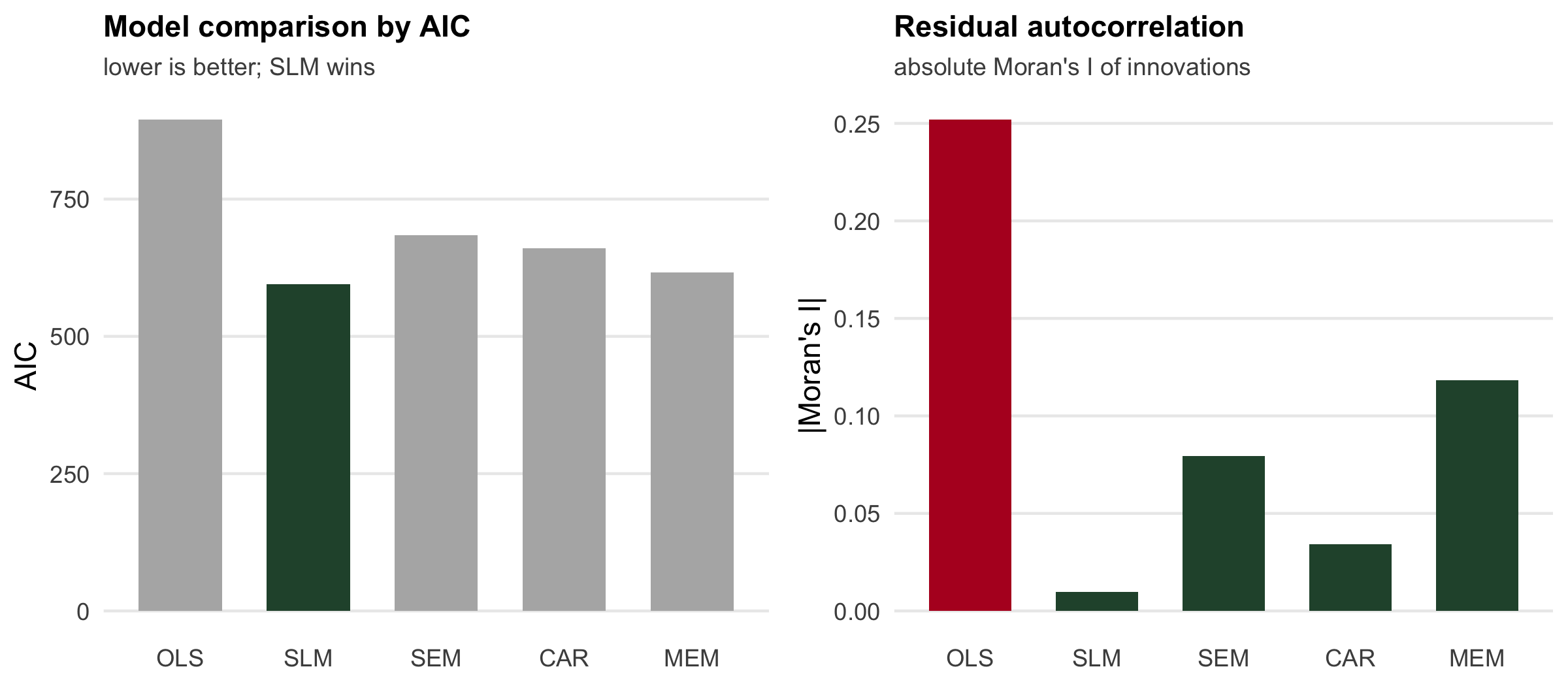
The verdict is unanimous with the LM tests. The spatial lag model wins on AIC, 595 against the naive 895, and it drives the residual Moran’s I to 0.01. The error and CAR models also whiten their innovations, but at a worse AIC, because they impose the wrong structure. The eigenvector filter whitens too, yet pays for 25 extra terms and lands in between. The lag test told us to expect a lag model; every global measure agrees.

The honest limit: spatial confounding

Now the caution. Suppose the covariate you care about is itself spatially smooth, as environmental drivers usually are. Adding a flexible spatial term, whether an eigenvector basis, an ICAR effect, or an error structure, gives the model a second way to describe smooth spatial variation. The covariate and the spatial term then compete for the same signal. Hodges and Reich (2010) showed that this inflates the variance of the fixed effect, and can shift the estimate itself. We reproduce the effect by adding progressively more eigenvector maps to a regression with a smooth spatial covariate that has a true slope of 0.6.

set.seed(4235)
xs  <- as.numeric(scale(sin(pi * coords$col / 13) * cos(pi * coords$row / 11) +
                        0.15 * rnorm(n)))            # a very smooth spatial covariate
b1c <- 0.6
ys  <- b0 + b1c * xs + as.numeric(solve(diag(n) - 0.6 * W) %*% rnorm(n, 0, 0.5))
Ks  <- c(0, 10, 30, 60, 100, 150); bx <- sx <- vif <- numeric(length(Ks))
for (i in seq_along(Ks)) {
  K <- Ks[i]
  if (K == 0) { m <- lm(ys ~ xs); vif[i] <- 1 } else {
    m <- lm(ys ~ xs + E[, broad[1:K]])
    vif[i] <- 1 / (1 - summary(lm(xs ~ E[, broad[1:K]]))$r.squared)
  }
  bx[i] <- coef(m)["xs"]; sx[i] <- summary(m)$coefficients["xs", "Std. Error"]
}
chk_bx <- bx; chk_sx <- sx; chk_vif <- vif
data.frame(maps = Ks, beta_x = round(bx, 3), se = round(sx, 3), VIF = round(vif, 1))

  maps beta_x    se  VIF
1    0  0.619 0.028  1.0
2   10  0.627 0.049  3.2
3   30  0.558 0.062  5.6
4   60  0.613 0.072  9.2
5  100  0.627 0.075 11.6
6  150  0.576 0.081 15.0

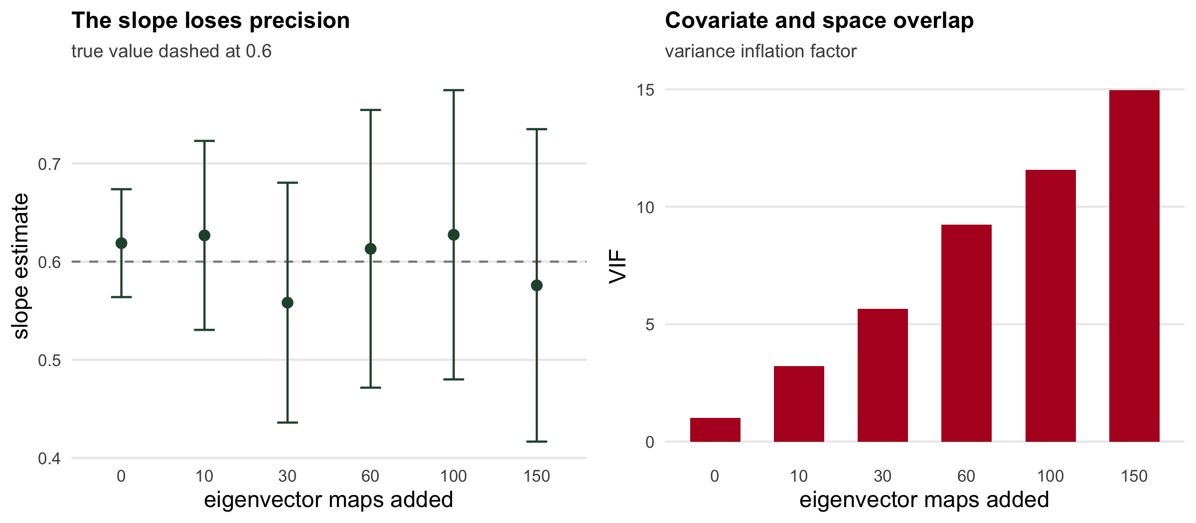
As more maps enter, the covariate becomes increasingly collinear with the spatial basis: its variance inflation factor climbs from 1 to 15. The standard error of the slope nearly triples, from 0.028 to 0.081, even though the point estimate stays near the true 0.6. You do not lose the estimate here, but you lose precision, badly, and with a smoother covariate or a more flexible spatial term the estimate itself starts to drift. “Controlling for space” is not free: past a point, the model can no longer tell whether the covariate or the map explains the pattern. This is the same collinearity that concurvity describes for additive models, now wearing a spatial coat.

What to carry forward

Checking an areal spatial model is a three-part routine. Read the residual Moran’s I on the innovations to confirm the autocorrelation is gone. Use the Lagrange multiplier tests to choose between a lag and an error specification, and back them with an AIC comparison across the model families. Then, before you report the covariate effect, ask whether it is still identified: if the predictor is spatially smooth, the spatial term will compete with it, inflating its standard error and possibly biasing it.

The remedy Hodges and Reich propose is restricted spatial regression, which confines the spatial term to the part of the map orthogonal to the fixed effects, so that space cannot steal the covariate’s signal. Whether that is the right choice depends on your question (Paciorek 2010), and there is no universal fix. The honest summary of this whole series is that spatial models repair the inference that autocorrelation breaks, but they introduce a tension of their own between explaining space and estimating effects. Diagnosing that tension, rather than assuming it away, is what separates a spatial analysis you can defend from one you cannot.

Related tutorials

• Spatial lag and spatial error models (SAR) fit the two models these tests choose between.
• Conditional autoregressive (CAR) models provide the CAR fit compared here.
• Moran eigenvector spatial filtering supplies the eigenvector basis used in the confounding demonstration.
• Concurvity in additive models is the non-spatial face of the same collinearity.

References

Anselin, L., Bera, A. K., Florax, R., & Yoon, M. J. (1996). Simple diagnostic tests for spatial dependence. Regional Science and Urban Economics, 26(1), 77-104. https://doi.org/10.1016/0166-0462(95)02111-6

Hodges, J. S., & Reich, B. J. (2010). Adding spatially-correlated errors can mess up the fixed effect you love. The American Statistician, 64(4), 325-334. https://doi.org/10.1198/tast.2010.10052

Paciorek, C. J. (2010). The importance of scale for spatial-confounding bias and precision of spatial regression estimators. Statistical Science, 25(1), 107-125.

Ver Hoef, J. M., Peterson, E. E., Hooten, M. B., Hanks, E. M., & Fortin, M.-J. (2018). Spatial autoregressive models for statistical inference from ecological data. Ecological Monographs, 88(1), 36-59. https://doi.org/10.1002/ecm.1283

## References

Anselin L, Bera AK, Florax R, Yoon MJ 1996 Regional Science and Urban Economics 26(1):77-104 (10.1016/0166-0462(95)02111-6)
Hodges JS, Reich BJ 2010 The American Statistician 64(4):325-334 (10.1198/tast.2010.10052)
Paciorek CJ 2010 Statistical Science 25(1):107-125 (10.1214/10-STS326)