side <- 20; n <- side * side
coords <- expand.grid(col = 1:side, row = 1:side)
A <- matrix(0, n, n)
idx <- function(r, c) (c - 1) * side + r
for (r in 1:side) for (c in 1:side) {
  i <- idx(r, c)
  if (r > 1)    A[i, idx(r - 1, c)] <- 1
  if (r < side) A[i, idx(r + 1, c)] <- 1
  if (c > 1)    A[i, idx(r, c - 1)] <- 1
  if (c < side) A[i, idx(r, c + 1)] <- 1
}
deg <- rowSums(A)          # number of neighbours per cell
W <- A / deg # row-standardised weightsSpatial lag and spatial error models (SAR)
spatial
regression
autocorrelation
areal data
ecology tutorial
Fit simultaneous autoregressive models to areal ecological data by hand, separate spillover from nuisance autocorrelation, and read the spatial multiplier.
Corrected 7 October 2026: the post set the error model’s slope aside as close enough to the truth, and its closing claim that the simulation shows the cost of fitting the wrong model rested on a simulation that never fitted it; the simulation now fits the error model too, and the text reports that it understates the slope and that its interval covers the truth far less often than it should.
Corrected 30 September 2026: the post read the AIC gap between the lag and error models as the data showing that the autocorrelation is a process; it now says the gap shows a better fit, expected here because the data were simulated from a spillover process, and that with real data an omitted spatial covariate can produce the same preference.
Updated 25 September 2026: a new section, When the neighbour rule is wrong, refits the lag model with queen and distance-band weights, and the closing caution now says what a wrong rule does to the coefficient and to the effects.
Count a species across a grid of survey cells, or average a trait across administrative regions, and you have areal data: one value per polygon, with a neighbourhood structure linking touching units. Ordinary least squares treats those cells as independent. They rarely are. Neighbouring cells share climate, share dispersers, share history, and so their residuals travel together. We met this problem for point locations in the Moran’s I tutorial and handled continuous-distance correlation with generalised least squares. Here the geometry is a lattice, and the natural tools are the simultaneous autoregressive (SAR) models: the spatial lag model and the spatial error model.
The two models look similar and are often confused, but they say different things about the world. One describes a process that spills across boundaries; the other describes a nuisance that merely clusters. Getting the distinction right changes both your coefficients and their standard errors, so this tutorial builds both from the likelihood up, in base R, and shows what ordinary least squares gets wrong.
The lattice and its weights
Everything starts from a neighbourhood. We use a regular 20 by 20 grid and rook contiguity: two cells are neighbours if they share an edge. The adjacency matrix A holds a 1 for every neighbour pair. Dividing each row by its number of neighbours gives the row-standardised weights matrix W, so that W %*% y returns, for every cell, the average of its neighbours.
The likelihood needs the eigenvalues of W. Because W is similar to a symmetric matrix, its eigenvalues are real and fall in the interval from minus one to one, which also fixes the admissible range of the autocorrelation parameter.
ev <- eigen(diag(1 / sqrt(deg)) %*% A %*% diag(1 / sqrt(deg)), symmetric = TRUE)$values
rho_lo <- 1 / min(ev); rho_hi <- 1 / max(ev)
range(ev)
[1] -1 1A reusable Moran’s I
We lean on Moran’s I throughout, so here is a compact base R version returning the statistic and its analytic p-value under the randomisation assumption. It matches the value from the spdep package exactly.
moran_test <- function(z, W) {
  n <- length(z); z <- z - mean(z)
  S0 <- sum(W); S1 <- 0.5 * sum((W + t(W))^2)
  S2 <- sum((rowSums(W) + colSums(W))^2)
  I  <- (n / S0) * as.numeric(t(z) %*% W %*% z) / sum(z^2)
  EI <- -1 / (n - 1); b2 <- n * sum(z^4) / (sum(z^2)^2)
  VI <- (n * ((n^2 - 3 * n + 3) * S1 - n * S2 + 3 * S0^2)
         - b2 * ((n^2 - n) * S1 - 2 * n * S2 + 6 * S0^2)) /
        ((n - 1) * (n - 2) * (n - 3) * S0^2) - EI^2
  list(I = I, p = pnorm((I - EI) / sqrt(VI), lower.tail = FALSE))
}
Two models, two stories
Write X for the design matrix holding an intercept and one covariate, and beta for the coefficients. The spatial lag model places the neighbour average of the response on the right-hand side:
\[ y = \rho W y + X\beta + \varepsilon. \]
Solving for y gives the reduced form y = (I - rho W)^{-1}(X beta + eps). The inverse (I - rho W)^{-1} is the spatial multiplier: a nudge to one cell propagates to its neighbours, then their neighbours, and so on. This is a model of a genuine process, dispersal, contagion, competition, that crosses cell boundaries.
The spatial error model puts the autocorrelation in the disturbance instead:
\[ y = X\beta + u, \qquad u = \lambda W u + \varepsilon. \]
Here the neighbourhood structure is a nuisance. The mean model X beta is what you care about; the clustered errors only spoil the standard errors. Both models are estimated by maximum likelihood. The only awkward term is the log-determinant of I - rho W, and the eigenvalues of W make that cheap; once it is available a general-purpose optimiser can search the parameters directly.
Simulating a spillover process
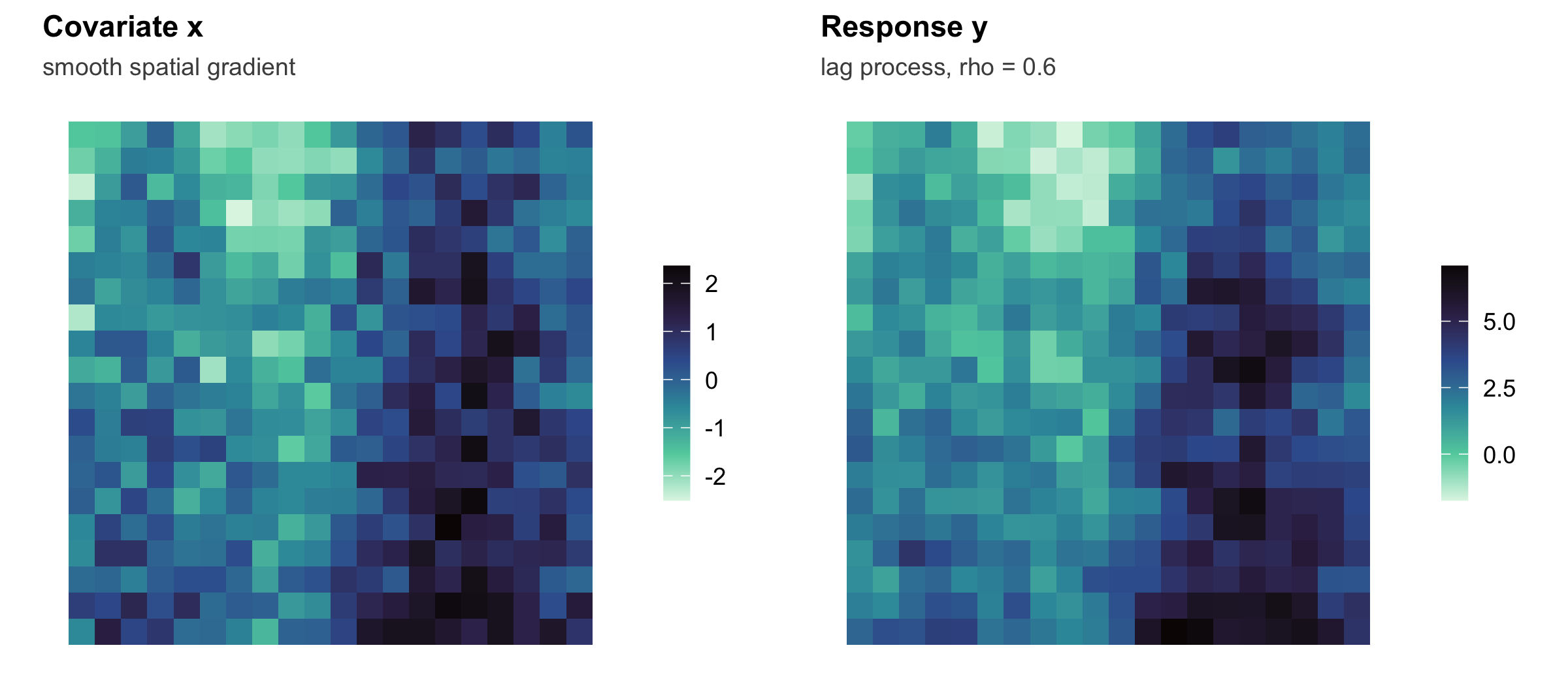
We generate data from the lag process with a modest spatial covariate, an autocorrelation of rho = 0.6, and a real slope of b1 = 0.8.
set.seed(4230)
cc <- scale(coords$col)[, 1]; rr <- scale(coords$row)[, 1]
x  <- as.numeric(scale(0.9 * sin(pi * coords$col / 6) + 0.7 * cc - 0.5 * rr +
                       rnorm(n, 0, 0.6)))
X  <- cbind(1, x)
b0 <- 1.0; b1 <- 0.8; rho <- 0.6; sig <- 0.5
Ainv <- solve(diag(n) - rho * W)
y <- as.numeric(Ainv %*% (X %*% c(b0, b1) + rnorm(n, 0, sig)))
Where ordinary least squares fails
Fit the naive regression and look at its residuals.
ols <- lm(y ~ x)
sar_ols_int   <- coef(ols)[1]
sar_ols_slope <- coef(ols)["x"]
sar_mi_ols <- moran_test(resid(ols), W)$I
sar_mp_ols <- moran_test(resid(ols), W)$p
round(c(intercept = sar_ols_int, slope = sar_ols_slope), 3)
intercept.(Intercept) slope.x
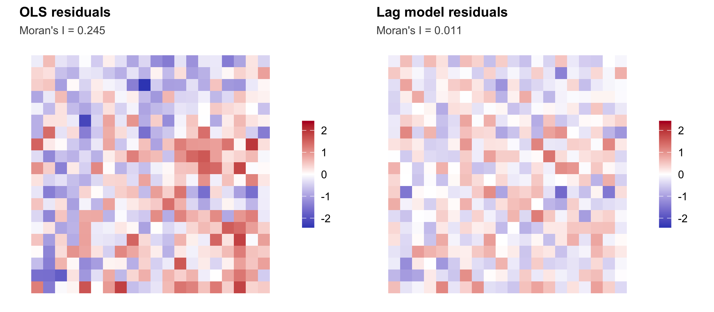
2.502 1.671 The true slope is 0.8, but ordinary least squares returns 1.67: more than double, because the omitted term rho W y is correlated with x through the multiplier and its pull is absorbed into the slope. The residuals carry a Moran’s I of 0.245 (p around \(4.9 \times 10^{-12}\)), so the independence assumption is plainly violated. Neither the coefficient nor its standard error can be trusted.
The spatial lag model by hand
The log-likelihood for the lag model, at a candidate rho, filters the response with A(rho) = I - rho W, scores the residuals A(rho) y - X beta, and adds the log-determinant log|I - rho W|, which the eigenvalues make cheap. Nothing is concentrated out: optim searches over the two coefficients, rho and the error scale together.
nll_lag <- function(par) {
  be <- par[1:2]; r <- par[3]; s2 <- exp(2 * par[4])
  if (r <= rho_lo || r >= rho_hi) return(1e10)
  Ay <- y - r * (W %*% y)
  e  <- Ay - X %*% be
  -(-n / 2 * log(2 * pi) - n / 2 * log(s2) +
      sum(log(1 - r * ev)) - sum(e^2) / (2 * s2))
}
fit_lag <- optim(c(coef(ols), 0.1, log(sd(resid(ols)))), nll_lag,
                 method = "BFGS", hessian = TRUE)
stopifnot(fit_lag$convergence == 0)   # check before inverting the Hessian
se_lag <- sqrt(diag(solve(fit_lag$hessian)))
sar_slm_b0    <- fit_lag$par[1]; sar_slm_b1  <- fit_lag$par[2]
sar_slm_rho   <- fit_lag$par[3]; sar_slm_serho <- se_lag[3]
sar_slm_sigma <- exp(fit_lag$par[4])
sar_slm_ll    <- -fit_lag$value
sar_slm_aic   <- 2 * 4 + 2 * fit_lag$value
sar_mi_slm    <- moran_test(as.numeric((diag(n) - sar_slm_rho * W) %*% y -
                                       X %*% fit_lag$par[1:2]), W)$I
data.frame(estimate = round(c(b0 = sar_slm_b0, b1 = sar_slm_b1,
                              rho = sar_slm_rho, sigma = sar_slm_sigma), 4))
estimate
b0.(Intercept) 1.0141
b1.x 0.8168
rho 0.5946
sigma 0.4949The estimates land on the truth: rho of 0.595 against 0.6, a slope of 0.817 against 0.8, and an intercept of 1.01 against 1. These match lagsarlm from the spatialreg package (it lived in spdep until the model-fitting code was split out) to within numerical precision. The filtered residuals now carry a Moran’s I of only 0.011, so the spatial structure has been accounted for rather than left in the errors.
Reading the spatial multiplier
In a plain regression, a one-unit change in x shifts the response by the slope, full stop. In a lag model the effect ripples outward, so the total effect is larger than the coefficient. The impact matrix (I - rho W)^{-1} b1 splits into a direct effect (the average change in a cell from its own covariate, including feedback loops), an indirect effect (the spillover onto other cells), and their sum.
M <- solve(diag(n) - sar_slm_rho * W) * sar_slm_b1
sar_direct   <- mean(diag(M))
sar_total    <- mean(rowSums(M))
sar_indirect <- sar_total - sar_direct
round(c(direct = sar_direct, indirect = sar_indirect, total = sar_total), 3)
direct indirect total
0.915 1.100 2.015 The direct effect, 0.92, sits just above the coefficient because of feedback through the neighbourhood. The indirect effect, 1.1, is the spillover, and it is larger than the direct part here. The total, 2.01, equals the tidy closed form b1 / (1 - rho) exactly, since each row of the multiplier sums to 1 / (1 - rho) for row-standardised weights. Reporting only the coefficient would understate the ecological effect by more than half. This decomposition is the single most important reason to prefer a lag model when the process really does cross boundaries.
The spatial error model, and why it is the wrong fit here
Fit the error model to the same data. Its concentrated likelihood filters both sides by B(lambda) = I - lambda W and runs generalised least squares.
nll_err <- function(par) {
  lam <- par[1]; s2 <- exp(2 * par[2])
  if (lam <= rho_lo || lam >= rho_hi) return(1e10)
  B <- diag(n) - lam * W; BtB <- crossprod(B)
  be <- solve(t(X) %*% BtB %*% X, t(X) %*% BtB %*% y)
  e  <- B %*% (y - X %*% be)
  -(-n / 2 * log(2 * pi) - n / 2 * log(s2) +
      sum(log(1 - lam * ev)) - sum(e^2) / (2 * s2))
}
fit_err <- optim(c(0.1, log(sd(resid(ols)))), nll_err, method = "BFGS")
lam_hat <- fit_err$par[1]
Bh <- diag(n) - lam_hat * W; BtB <- crossprod(Bh)
be_err <- solve(t(X) %*% BtB %*% X, t(X) %*% BtB %*% y)
sar_sem_lambda <- lam_hat; sar_sem_b1 <- be_err[2]
sar_sem_aic <- 2 * 4 + 2 * fit_err$value
round(c(lambda = sar_sem_lambda, b1 = sar_sem_b1, AIC = sar_sem_aic), 3)
lambda b1 AIC
0.894 0.748 722.758 The error model reaches for a large lambda of 0.89 to mop up the leftover structure, and its slope of 0.75 is close to the true 0.8 in this dataset, although the simulation below shows that over repeated draws the error model’s slope runs low and its interval covers the true slope far less often than it should. The larger problem is what the output does not contain: no multiplier, so no spillover of 1.1 and no total effect of 2.01, and a reader would take the coefficient as the whole story. Its AIC of 723 is also far worse than the lag model’s 623, and that gap says the lag specification describes these data far better, which is what we expect because we simulated a spillover process. With real data a better fit is consistent with a process but does not prove one, since an omitted, spatially structured covariate can produce the same preference. On data actually generated by an error process the verdict would usually flip. Deciding between the two from data, rather than assuming, is the job of the formal tests in checking a spatial regression.
How much does it matter? A short simulation
One dataset can mislead. We repeat the whole exercise 400 times, comparing the ordinary least squares slope, the lag estimate and the error-model slope, and asking how often each ninety-five per cent interval actually covers the true slope.
set.seed(99); B <- 400
ols_b <- slm_b <- ols_cov <- slm_cov <- sem_b <- sem_cov <- numeric(B)
WX <- W %*% X
for (b in 1:B) {
  yb <- as.numeric(Ainv %*% (X %*% c(b0, b1) + rnorm(n, 0, sig)))
  o  <- lm(yb ~ x); ob <- coef(o)["x"]
  ose <- summary(o)$coefficients["x", "Std. Error"]
  ols_b[b] <- ob; ols_cov[b] <- (b1 >= ob - 1.96 * ose & b1 <= ob + 1.96 * ose)
  fl <- optim(c(coef(o), 0.1, log(sd(resid(o)))), function(par) {
    be <- par[1:2]; r <- par[3]; s2 <- exp(2 * par[4])
    if (r <= rho_lo || r >= rho_hi) return(1e10)
    Ay <- yb - r * (W %*% yb); e <- Ay - X %*% be
    -(-n / 2 * log(2 * pi) - n / 2 * log(s2) + sum(log(1 - r * ev)) - sum(e^2) / (2 * s2))
  }, method = "BFGS", hessian = TRUE)
  sb <- fl$par[2]; sse <- sqrt(diag(solve(fl$hessian)))[2]
  slm_b[b] <- sb; slm_cov[b] <- (b1 >= sb - 1.96 * sse & b1 <= sb + 1.96 * sse)
  # error model: the sem likelihood with beta and the error variance profiled out
  Wyb <- as.numeric(W %*% yb)
  lh <- optimize(function(l) n / 2 * log(sum(qr.resid(qr(X - l * WX), yb - l * Wyb)^2) / n) -
                   sum(log(1 - l * ev)), c(rho_lo + 1e-6, rho_hi - 1e-6))$minimum
  qe <- qr(X - lh * WX); eb <- qr.coef(qe, yb - lh * Wyb)[2]
  ese <- sqrt(sum(qr.resid(qe, yb - lh * Wyb)^2) / n * chol2inv(qr.R(qe))[2, 2])
  sem_b[b] <- eb; sem_cov[b] <- (b1 >= eb - 1.96 * ese & b1 <= eb + 1.96 * ese)
}
sar_mc_ols_bias <- 100 * (mean(ols_b) - b1) / b1
sar_mc_ols_cov  <- mean(ols_cov)
sar_mc_slm_bias <- 100 * (mean(slm_b) - b1) / b1
sar_mc_slm_cov  <- mean(slm_cov)
sar_mc_sem_bias <- 100 * (mean(sem_b) - b1) / b1
sar_mc_sem_cov  <- mean(sem_cov)
round(c(ols_bias_pct = sar_mc_ols_bias, ols_cover = sar_mc_ols_cov,
        slm_bias_pct = sar_mc_slm_bias, slm_cover = sar_mc_slm_cov,
        sem_bias_pct = sar_mc_sem_bias, sem_cover = sar_mc_sem_cov), 3)
ols_bias_pct ols_cover slm_bias_pct slm_cover sem_bias_pct sem_cover
108.085 0.000 0.716 0.940 -8.556 0.647 Ordinary least squares overstates the slope by 108 per cent on average, and its confidence interval covers the truth in 0 per cent of runs: a total failure of inference. The lag model is essentially unbiased, off by 0.7 per cent, with 94 per cent coverage, close to the nominal ninety-five. The error model, fitted to the same draws, understates the slope by 8.6 per cent on average, and its interval covers the truth in 65 per cent of runs: far better than ordinary least squares, but well short of the nominal level.
When the neighbour rule is wrong
Every number so far used the rook weights that generated the data. In a real analysis the rule is chosen, not known, and queen contiguity (corners count as neighbours) and distance bands are common alternatives. The chunk below takes fresh draws from the same lag process, still generated with rook weights, and fits the lag model to each draw three times: with rook weights, with queen weights, and with a band that joins every pair of cells closer than 2.9 cell widths. The fit is the same likelihood as above with the coefficients and the error variance profiled out, so only rho is searched numerically. The direct effect comes from the eigenvalues, because the mean diagonal element of (I - rho W)^{-1} is the mean of 1 / (1 - rho * ev).
d_cell <- as.matrix(dist(coords))
w_from <- function(adj) {
  nb <- rowSums(adj)
  list(W = adj / nb,
       ev = eigen(diag(1 / sqrt(nb)) %*% adj %*% diag(1 / sqrt(nb)),
                  symmetric = TRUE, only.values = TRUE)$values)
}
w_rules <- list(rook = w_from(A),
                queen = w_from((d_cell > 0 & d_cell < 1.5) * 1),
                band = w_from((d_cell > 0 & d_cell < 2.9) * 1))
nb_count <- sapply(list(A, (d_cell > 0 & d_cell < 1.5) * 1,
                        (d_cell > 0 & d_cell < 2.9) * 1),
                   function(adj) max(rowSums(adj)))

fit_lag_w <- function(yv, wr) {
  wy <- as.numeric(wr$W %*% yv)
  prof <- function(r) {
    e <- qr.resid(qr(X), yv - r * wy)
    n / 2 * log(sum(e^2) / n) - sum(log(1 - r * wr$ev))
  }
  opt <- optimize(prof, c(1 / min(wr$ev) + 1e-6, 1 - 1e-6))
  r <- opt$minimum
  bw <- qr.coef(qr(X), yv - r * wy)
  c(b1 = bw[2], rho = r, total = bw[2] / (1 - r),
    direct = bw[2] * mean(1 / (1 - r * wr$ev)),
    loglik = -opt$objective - n / 2 * (log(2 * pi) + 1))
}

set.seed(5117)
n_rep_w <- 400
w_sims <- replicate(n_rep_w, {
  yw <- as.numeric(Ainv %*% (X %*% c(b0, b1) + rnorm(n, 0, sig)))
  sapply(w_rules, function(wr) fit_lag_w(yw, wr))
})
row_nm <- c("b1", "rho", "total", "direct", "loglik")
w_med <- sapply(names(w_rules), function(k)
  apply(w_sims[, k, ], 1, median))
rownames(w_med) <- row_nm
w_tab <- data.frame(neighbours = nb_count,
                    slope_ratio = w_med["b1", ] / b1,
                    rho = w_med["rho", ],
                    total_ratio = w_med["total", ] / (b1 / (1 - rho)),
                    direct = w_med["direct", ],
                    indirect = w_med["total", ] - w_med["direct", ])
print(round(w_tab, 3))
neighbours slope_ratio rho total_ratio direct indirect
rook 4 1.012 0.596 0.996 0.907 1.085
queen 8 1.051 0.590 1.017 0.901 1.133
band 24 1.177 0.571 1.087 0.965 1.209w_best <- apply(w_sims[5, , ], 2, which.max)
w_pick_rook <- mean(w_best == 1)
w_ll_gap <- median(w_sims[5, "rook", ] - w_sims[5, "queen", ])
cat("share of replicates where rook has the highest log-likelihood:",
round(w_pick_rook, 3), " median log-likelihood gap, rook minus queen:",
round(w_ll_gap, 2), "\n")share of replicates where rook has the highest log-likelihood: 1 median log-likelihood gap, rook minus queen: 16.22 With the rook weights that made the data, the median slope over 400 draws is 1.012 times the truth and the median total effect 0.996 times the true b1 / (1 - rho). With queen weights the median slope is 5.1 per cent above the truth and the median total 1.7 per cent above it. With the band they are 17.7 and 8.7 per cent above. Under both wrong rules the coefficient moves more than the total effect, because a wider neighbourhood returns a smaller rho (median 0.571 for the band against 0.596 for rook) together with a larger slope, and the two errors partly cancel in b1 / (1 - rho).
This is the argument of LeSage and Pace (2014), demonstrated rather than discovered here: they trace the common belief that lag-model results are sensitive to W largely to reading the coefficients as if they were the effects, whereas the effects (the partial derivatives summarised as direct, indirect and total impacts) move less. Less is not nothing, though. The band still overstates the total by the amount above, and both parts of it grow: the direct effect from 0.907 under rook to 0.965, the spillover from 1.085 to 1.209.
The log-likelihood picks rook in 100 per cent of the draws, with a median lead of 16.2 log-likelihood units over queen, so here the data can tell the rules apart. That is the easy case: the rule that generated the data is one of the candidates, and rho is 0.6. With real data none of the candidate rules is the process itself, and the same comparison only ranks approximations to it.
What to carry forward
For areal data on a lattice, the choice is not whether to model space but how. A spatial lag model treats neighbourhood dependence as a process and rewards you with an interpretable multiplier that separates direct effects from spillover. A spatial error model treats it as a nuisance and simply repairs the standard errors. Fitting the wrong one, or fitting neither, distorts both estimates and inference, as the simulation makes plain.
Two honest cautions. Every result outside the section on a wrong neighbour rule assumes the neighbourhood matrix W is correct. That section shows a wrong rule moves the coefficient more than the effects, but it moves the effects too, and with real data the choice is rarely obvious. And these models assume the spatial dependence is stationary across the map. The conditional autoregressive models tutorial offers a different route to the same goal, built on local conditional distributions rather than a simultaneous system, and checking a spatial regression shows how to test which specification your data actually support and where even a good spatial model can quietly mislead you.
References
Anselin L 1988 Spatial Econometrics: Methods and Models. Kluwer (10.1007/978-94-015-7799-1)
Dormann CF, McPherson JM, Araujo MB, Bivand R, Bolliger J, Carl G, et al. 2007 Ecography 30(5):609-628 (10.1111/j.2007.0906-7590.05171.x)
Kissling WD, Carl G 2008 Global Ecology and Biogeography 17(1):59-71 (10.1111/j.1466-8238.2007.00334.x)
LeSage JP, Pace RK 2014 Econometrics 2(4):217-249 (10.3390/econometrics2040217)
Ver Hoef JM, Peterson EE, Hooten MB, Hanks EM, Fortin M-J 2018 Ecological Monographs 88(1):36-59 (10.1002/ecm.1283)