gp_field <- function(coords, range, nugget = 0) {
  d <- as.matrix(dist(coords))
  S <- exp(-d / range)
  diag(S) <- 1 + nugget
  as.vector(t(chol(S)) %*% rnorm(nrow(coords)))
}

set.seed(204)
n  <- 150
co <- data.frame(xc = runif(n, 0, 10), yc = runif(n, 0, 10))
canopy <- 50 + 15 * scale(gp_field(co, range = 3))[, 1]
cover  <- 10 + 0.5 * canopy + 8 * gp_field(co, range = 2.5, nugget = 0.15)
df <- data.frame(co, canopy = canopy, cover = cover)Generalised least squares for spatial data in R
R
GLS
spatial
regression
ecology tutorial
When regression residuals are spatially autocorrelated, OLS standard errors mislead. Fit a GLS model with nlme, pick a correlation structure by AIC, and compare.
Ordinary least squares assumes the residuals are independent. Field data rarely cooperates: plots close together tend to share unmeasured conditions (soil, drainage, microclimate), so their residuals look alike. The post on Moran’s I showed how to detect that dependence. This post is the remedy. Generalised least squares lets the residuals carry a spatial correlation structure, which corrects two problems that ordinary regression hides: standard errors that are too small, and, when a predictor is itself spatially patterned, coefficient estimates that are biased.
We will build a synthetic landscape so the truth is known, fit it both ways, and watch which estimator recovers the values used to generate the data.
The symptom
Fit ordinary least squares (gls with independent errors is identical to lm, and fitting it this way keeps every model on the same footing for later comparison) and map its residuals across the landscape.
m_ols <- gls(cover ~ canopy, data = df, method = "REML")
df$ols_resid <- residuals(m_ols, type = "response")
summary(m_ols)$tTable
Value Std.Error t-value p-value
(Intercept) 24.5295648 1.97538230 12.417629 1.040608e-24
canopy 0.2733377 0.03785188 7.221244 2.511352e-11ggplot(df, aes(xc, yc, colour = ols_resid)) +
geom_point(size = 3.4, alpha = 0.95) +
scale_colour_gradient2(low = "#b5534e", mid = "#e7e4d6", high = "#1d5b4e",
midpoint = 0, name = "OLS\nresidual") +
coord_equal() +
labs(x = "Easting", y = "Northing") +
base_theme + theme(legend.position = "right")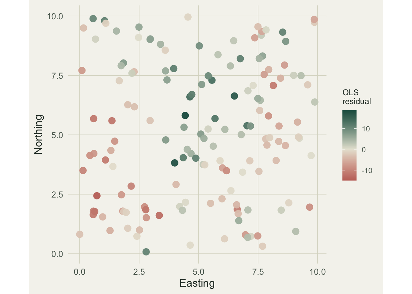
If the residuals were independent, this map would be a random wash of colours. Instead the greens and reds clump: positive residuals run through the centre, negative ones gather at the edges. A formal Moran’s I test (covered in the earlier post) would confirm it, but the eye is enough here. The independence assumption behind the OLS standard errors does not hold, so the p-values cannot be trusted.
The fix: a correlation structure on the residuals
gls from nlme fits the same linear model but lets you specify how residuals covary. corExp says the correlation between two plots decays exponentially with the distance between them; nugget = TRUE adds a share of variance that is not spatial, soaking up measurement error and fine-scale noise.
m_exp <- gls(cover ~ canopy, data = df, method = "REML",
             correlation = corExp(form = ~ xc + yc, nugget = TRUE))
summary(m_exp)$tTable
Value Std.Error t-value p-value
(Intercept) 13.1905550 3.77229633 3.496691 6.221073e-04
canopy 0.4627138 0.04444089 10.411894 2.175866e-19Compare the two fits against the values that generated the data (intercept 10, slope 0.5). OLS put the slope at 0.27 and the intercept at 24.5; GLS puts the slope at 0.46 and the intercept at 13.2. GLS is much closer to the truth on both. The reason is that OLS treated all 150 plots as independent evidence, when clusters of nearby plots are partly carrying the same information. Telling the model that, through the correlation structure, shrinks the effective sample size: it widens the standard errors (the intercept’s nearly doubles, from 2.0 to 3.8) and, because canopy is itself spatially patterned, it pulls the confounded slope back toward its real value. Under spatial autocorrelation, OLS is not just overconfident; its point estimates can be wrong.
The fitted structure has interpretable parts:
coef(m_exp$modelStruct$corStruct, unconstrained = FALSE) range nugget
2.3940610 0.1041068 The range, 2.4, is the distance over which correlation falls to about a third: plots closer than that are meaningfully linked, plots much farther apart are effectively independent. The nugget, 0.10, says about a tenth of the residual variance is non-spatial noise. A residual variogram shows the same thing: semivariance climbs with distance until it levels off at the sill, and the fitted exponential summarises that rise.
vg  <- Variogram(m_exp, resType = "response")
cs  <- coef(m_exp$modelStruct$corStruct, unconstrained = FALSE)
sig2 <- summary(m_exp)$sigma^2
curve_df <- data.frame(dist = seq(0.01, max(vg$dist), length.out = 200))
curve_df$gamma <- sig2 * (1 - (1 - cs[["nugget"]]) * exp(-curve_df$dist / cs[["range"]]))

ggplot() +
  geom_point(data = vg, aes(dist, variog), colour = forest, size = 2.4, alpha = 0.8) +
  geom_line(data = curve_df, aes(dist, gamma), colour = "#c9a13f", linewidth = 1) +
  geom_hline(yintercept = sig2, linetype = "dotted", colour = faint) +
  labs(x = "Distance between plots", y = "Semivariance of residuals") +
  base_theme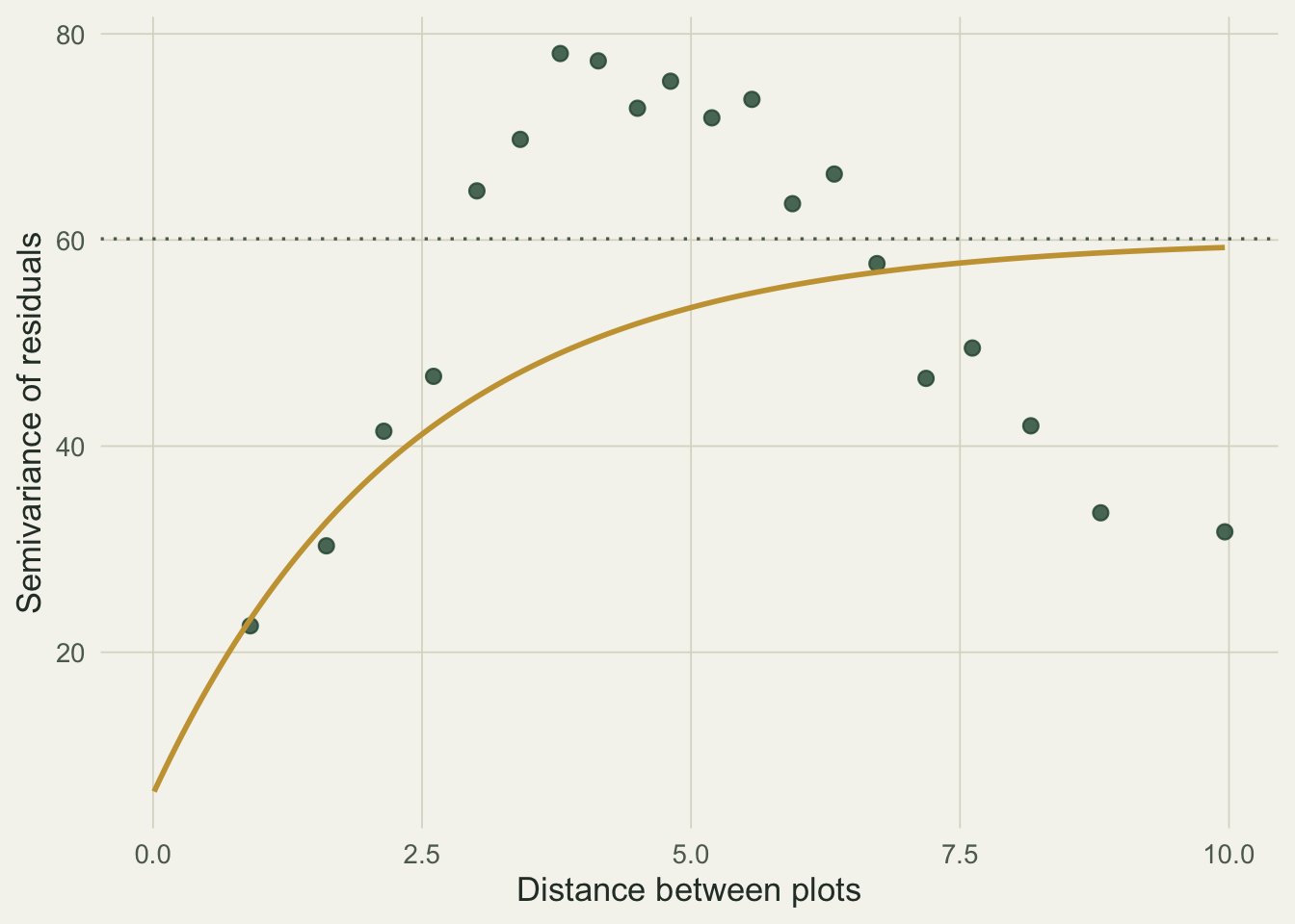
Choosing the structure
corExp is one option among several. corGaus decays as a Gaussian (smoother fields), corSpher reaches independence at a finite distance. Fit the candidates and compare them, along with the independent-errors model, by AIC.
m_gau <- update(m_exp, correlation = corGaus(form = ~ xc + yc, nugget = TRUE))
m_sph <- update(m_exp, correlation = corSpher(form = ~ xc + yc, nugget = TRUE))
AIC(m_ols, m_exp, m_gau, m_sph)
df AIC
m_ols 3 1014.4773
m_exp 5 911.6535
m_gau 5 920.2874
m_sph 5 910.9282Two things stand out. Any spatial structure beats the independent-errors model by about 100 AIC units: an overwhelming preference for modelling the autocorrelation at all. Among the spatial structures the gap is small. Exponential and spherical are within one AIC unit of each other (indistinguishable on this evidence), and Gaussian trails by about nine. The practical lesson is that the decision that matters is whether to model spatial correlation, not which decay shape you choose; pick the best by AIC, but do not agonise between exponential and spherical when they tie. Comparing correlation structures this way uses REML, which is the default; switch to method = "ML" only when you are comparing models with different fixed effects.
Why it is worth the trouble
The cost of ignoring autocorrelation is not abstract. Simulate the null case: a predictor with no real effect on the response, but both the predictor and the residuals spatially structured, fitted both ways one hundred and fifty times, counting how often each method declares the slope significant at 0.05. With a true slope of zero, every rejection is a false positive.
set.seed(771)
nsim <- 150; nn <- 100
cs2 <- data.frame(xc = runif(nn, 0, 10), yc = runif(nn, 0, 10))
dd  <- as.matrix(dist(cs2))
Lx <- t(chol({ S <- exp(-dd / 3);   diag(S) <- 1;        S }))
Le <- t(chol({ S <- exp(-dd / 2.5); diag(S) <- 1 + 0.15; S }))

res <- t(replicate(nsim, {
  xf <- 50 + 15 * scale(Lx %*% rnorm(nn))[, 1]
  yf <- 10 + 0 * xf + 8 * (Le %*% rnorm(nn))[, 1]   # true slope is zero
  p_ols <- summary(lm(yf ~ xf))$coefficients["xf", "Pr(>|t|)"]
  p_gls <- tryCatch(
    summary(gls(yf ~ xf, data = data.frame(cs2, xf, yf),
                correlation = corExp(form = ~ xc + yc, nugget = TRUE)))$tTable["xf", "p-value"],
    error = function(e) NA_real_)
  c(ols = p_ols, gls = p_gls)
}))
ok <- !is.na(res[, "gls"])
c(OLS = mean(res[ok, "ols"] < 0.05), GLS = mean(res[ok, "gls"] < 0.05))
OLS GLS
0.33557047 0.08724832 td <- data.frame(method = factor(c("OLS", "GLS"), levels = c("OLS", "GLS")),
rate = c(mean(res[ok, "ols"] < 0.05), mean(res[ok, "gls"] < 0.05)))
ggplot(td, aes(method, rate, fill = method)) +
geom_col(width = 0.55) +
geom_hline(yintercept = 0.05, linetype = "dashed", colour = "#b5534e", linewidth = 0.6) +
geom_text(aes(label = sprintf("%.1f%%", 100 * rate)), vjust = -0.5, colour = body, size = 4.4) +
annotate("text", x = 2.48, y = 0.058, label = "nominal 5%",
colour = "#b5534e", size = 3.3, hjust = 1) +
scale_fill_manual(values = c(OLS = "#b5534e", GLS = "#275139")) +
scale_y_continuous(expand = expansion(mult = c(0, 0.12)),
labels = function(x) paste0(x * 100, "%")) +
labs(x = NULL, y = "False-positive rate (true slope = 0)") +
base_theme + theme(legend.position = "none")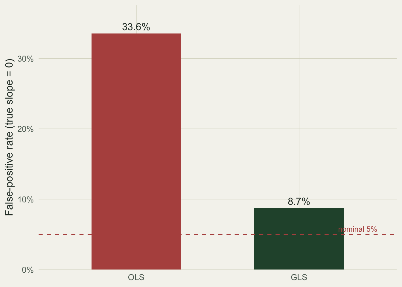
Ordinary least squares calls a non-existent effect significant about a third of the time, nearly seven times the rate it advertises. GLS pulls that back close to 5 percent. The handful of points by which it overshoots is the usual price of estimating the correlation parameters from the same data; it is a rounding error next to the OLS inflation.
A few practical notes. gls is for continuous, roughly Gaussian responses. For counts or presence-absence with spatial dependence, the analogue is a spatial term inside a mixed model or a spatial smooth inside a GAM. Start with corExp and a nugget, read the range to judge the scale of dependence, and always compare against the independent-errors model so you can see what the correction buys you.
References
Pinheiro and Bates 2000 Mixed-Effects Models in S and S-PLUS, Springer (10.1007/b98882).
Zuur, Ieno, Walker, Saveliev and Smith 2009 Mixed Effects Models and Extensions in Ecology with R, Springer (10.1007/978-0-387-87458-6).
Dormann et al. 2007 Ecography 30(5):609-628 (10.1111/j.2007.0906-7590.05171.x).
Legendre 1993 Ecology 74(6):1659-1673 (10.2307/1939924).