Conditional autoregressive (CAR) models

Build areal spatial dependence from local conditional distributions, fit a proper CAR by hand, contrast it with SAR, and use the intrinsic CAR as a smoother.

Corrected 7 October 2026: the right-hand map of the first figure was still titled a proper-CAR field after its caption was corrected; its title now calls it the simulated response, covariate plus proper-CAR error; the heading of the section that compares the two models also still said that a CAR is not a SAR in disguise, the general claim an earlier correction withdrew, and it now names what the section compares, a CAR and a SAR built on the same neighbours.

Corrected 1 October 2026: the caption of the first figure presented its right-hand map as the CAR field without saying that most of its pattern comes from the covariate, and the text description of the smoothing figure said the noise was removed when part of it remains; both now describe the maps as they are.

Corrected 30 September 2026: the post said, citing Ver Hoef and colleagues, that neither a CAR nor a SAR is a reparametrisation of the other except in special cases; either can in fact be rewritten as the other with different neighbour weights, and the post now says that the two differ when built on the same neighbourhood matrix.

The simultaneous autoregressive models build spatial dependence from the top down: one global equation, y = rho W y + X beta + eps, solved all at once. Conditional autoregressive (CAR) models take the opposite route. They specify, for each cell, only its distribution given its neighbours, and let a theorem stitch those local pieces into a coherent joint distribution. This bottom-up construction, due to Besag (1974), is the engine behind most Bayesian disease mapping and behind the spatial random effects in ecological hierarchical models. It is worth understanding directly.

This tutorial writes the conditional model down, assembles its precision matrix, fits a proper CAR by hand in base R, and then does three things the textbooks often skip: it shows why the CAR autocorrelation parameter is not comparable across software packages, it contrasts the covariance a CAR implies with the one a SAR implies, and it uses the intrinsic CAR as a practical smoother.

The conditional specification

A CAR model says that, conditional on every other cell, cell i is normal with a mean pulled towards its neighbours:

\[ y_i \mid y_{-i} \sim \mathcal{N}\!\left(\mu_i + \rho \sum_j \frac{a_{ij}}{d_i}(y_j - \mu_j),\ \frac{\tau^2}{d_i}\right), \]

where a_ij marks neighbours, d_i is the number of neighbours of cell i, and mu = X beta. The Hammersley-Clifford theorem guarantees these conditionals correspond to a single joint Gaussian, and its precision matrix (the inverse covariance) is wonderfully sparse:

\[ Q = \frac{1}{\tau^2}(D - \rho A), \]

with D the diagonal matrix of neighbour counts and A the adjacency matrix. The model is proper (a valid distribution) when D - rho A is positive definite, which pins rho inside a range set by the eigenvalues.

Setting up the lattice

side <- 20; n <- side * side
coords <- expand.grid(col = 1:side, row = 1:side)
A <- matrix(0, n, n)
idx <- function(r, c) (c - 1) * side + r
for (r in 1:side) for (c in 1:side) {
  i <- idx(r, c)
  if (r > 1)    A[i, idx(r - 1, c)] <- 1
  if (r < side) A[i, idx(r + 1, c)] <- 1
  if (c > 1)    A[i, idx(r, c - 1)] <- 1
  if (c < side) A[i, idx(r, c + 1)] <- 1
}
deg <- rowSums(A); D <- diag(deg)
# eigenvalues of the row-standardised operator fix the admissible rho range
ev <- eigen(diag(1 / sqrt(deg)) %*% A %*% diag(1 / sqrt(deg)), symmetric = TRUE)$values
rho_lo <- 1 / min(ev); rho_hi <- 1 / max(ev)
c(lower = rho_lo, upper = rho_hi)

lower upper 
   -1     1 

Simulating a proper CAR field

We draw one realisation with an intercept, a covariate, a strong conditional dependence of rho = 0.9, and a conditional scale of tau = 0.4. Sampling is direct from the joint covariance tau^2 (D - rho A)^{-1}.

set.seed(4231)
cc <- scale(coords$col)[, 1]
x  <- as.numeric(scale(0.8 * cos(pi * coords$row / 7) + 0.6 * cc + rnorm(n, 0, 0.6)))
X  <- cbind(1, x)
b0 <- 0.5; b1 <- 0.7; rho <- 0.9; tau <- 0.4
Q  <- (D - rho * A) / tau^2
set.seed(11)
y  <- as.numeric(X %*% c(b0, b1) + t(chol(solve(Q))) %*% rnorm(n))

Fitting a CAR by hand

The log-likelihood needs the log-determinant of the precision. Factor it as |D - rho A| = |D| * |I - rho D^{-1}A|, so the determinant reduces to a sum over the same eigenvalues we already have. For each candidate rho we solve the generalised least squares problem for beta, read off tau from the quadratic form, and search over the single remaining parameter.

nll_car <- function(r) {
  if (r <= rho_lo || r >= rho_hi) return(1e10)
  P  <- D - r * A                               # precision up to 1/tau^2
  be <- solve(t(X) %*% P %*% X, t(X) %*% P %*% y)
  e  <- y - X %*% be; t2 <- as.numeric(t(e) %*% P %*% e) / n
  ldetP <- sum(log(deg)) + sum(log(1 - r * ev)) # log|D - rho A|
  -(-n / 2 * log(2 * pi) - n / 2 - n / 2 * log(t2) + 0.5 * ldetP)
}
opt <- optimise(nll_car, c(rho_lo + 1e-4, rho_hi - 1e-4))
car_rho <- opt$minimum
P  <- D - car_rho * A
be <- solve(t(X) %*% P %*% X, t(X) %*% P %*% y)
car_b0 <- be[1]; car_b1 <- be[2]
car_tau <- sqrt(as.numeric(t(y - X %*% be) %*% P %*% (y - X %*% be)) / n)
car_ll  <- -opt$objective
round(c(rho = car_rho, tau = car_tau, b0 = car_b0, b1 = car_b1), 4)

   rho    tau     b0     b1 
0.8184 0.3929 0.4774 0.6893 

The fit recovers the generating values well: a conditional dependence of 0.82 against the true 0.9, a scale of 0.39 against 0.4, and a slope of 0.69 against 0.7. The likelihood machinery is the same log-determinant plus generalised least squares we used for the error model in the SAR tutorial, only the precision differs.

A warning about conventions

Reach for a package and you may be surprised. The spautolm function in spatialreg (it lived in spdep before the model-fitting code was split out), with family = "CAR", does not use the neighbour-count precision D - rho A. It uses a symmetric-weights convention, which with binary weights gives the precision I - lambda A. That is a different model, so its lambda is not on the same scale as our rho and the two numbers will never agree. To show this is a convention and not an error, we can fit the symmetric version by hand as well.

evA <- eigen(A, symmetric = TRUE)$values
loA <- 1 / min(evA); hiA <- 1 / max(evA)
nll_sym <- function(lam) {
  if (lam <= loA || lam >= hiA) return(1e10)
  P  <- diag(n) - lam * A
  be <- solve(t(X) %*% P %*% X, t(X) %*% P %*% y); e <- y - X %*% be
  s2 <- as.numeric(t(e) %*% P %*% e) / n
  -(-n / 2 * log(2 * pi) - n / 2 - n / 2 * log(s2) + 0.5 * sum(log(1 - lam * evA)))
}
car_sym_lambda <- optimise(nll_sym, c(loA + 1e-6, hiA - 1e-6))$minimum
round(car_sym_lambda, 4)

[1] 0.2122

The symmetric convention reports 0.212, and this by-hand value matches spatialreg’s spautolm to numerical precision. It is fitted to the same data as our 0.82, but under a different model, with a parameter on a different scale. The lesson is practical: never compare a CAR autocorrelation parameter across papers or packages without first checking which weights convention each one uses.

CAR and SAR on the same neighbours

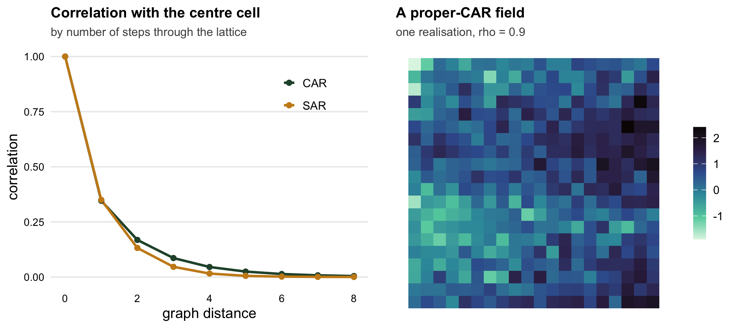
Both models encode neighbourhood dependence, but built on the same neighbourhood matrix they imply different covariances (Ver Hoef et al. 2018 compare the two families); rewriting one as the other means changing the neighbour weights. A useful way to see the difference is to trace how the correlation between a central cell and the rest decays with graph distance, the number of steps through the lattice.

centre <- idx(10, 10)
gdist  <- rep(NA_integer_, n); gdist[centre] <- 0L; step <- 0L; front <- centre
repeat {
  nb <- setdiff(unique(unlist(lapply(front, function(i) which(A[i, ] > 0)))),
                which(!is.na(gdist)))
  if (!length(nb)) break
  step <- step + 1L; gdist[nb] <- step; front <- nb
}
Ccar <- cov2cor(solve(D - 0.9 * A))[centre, ]                       # CAR reach
Wrs  <- A / deg
Csar <- cov2cor(solve(crossprod(diag(n) - 0.6 * Wrs)))[centre, ]    # SAR reach
reach <- aggregate(data.frame(CAR = Ccar, SAR = Csar), list(dist = gdist), mean)
round(head(reach, 5), 3)

  dist   CAR   SAR
1    0 1.000 1.000
2    1 0.346 0.350
3    2 0.168 0.132
4    3 0.086 0.046
5    4 0.045 0.016

At the first step the two are tuned to match, near 0.35. Further out they part company: at three steps the CAR retains a correlation of 0.086 against the SAR’s 0.046. The conditional model here carries dependence further across the map than the simultaneous one at matched short range. Which shape suits your system is an empirical question, and one more reason the two model families are worth keeping distinct.

Correlation with the centre cell against graph distance for a CAR and a SAR tuned to match at one step (left), and one realisation of the simulated response on the lattice, covariate plus proper-CAR error, most of whose visible pattern comes from the covariate (right).

The intrinsic CAR as a smoother

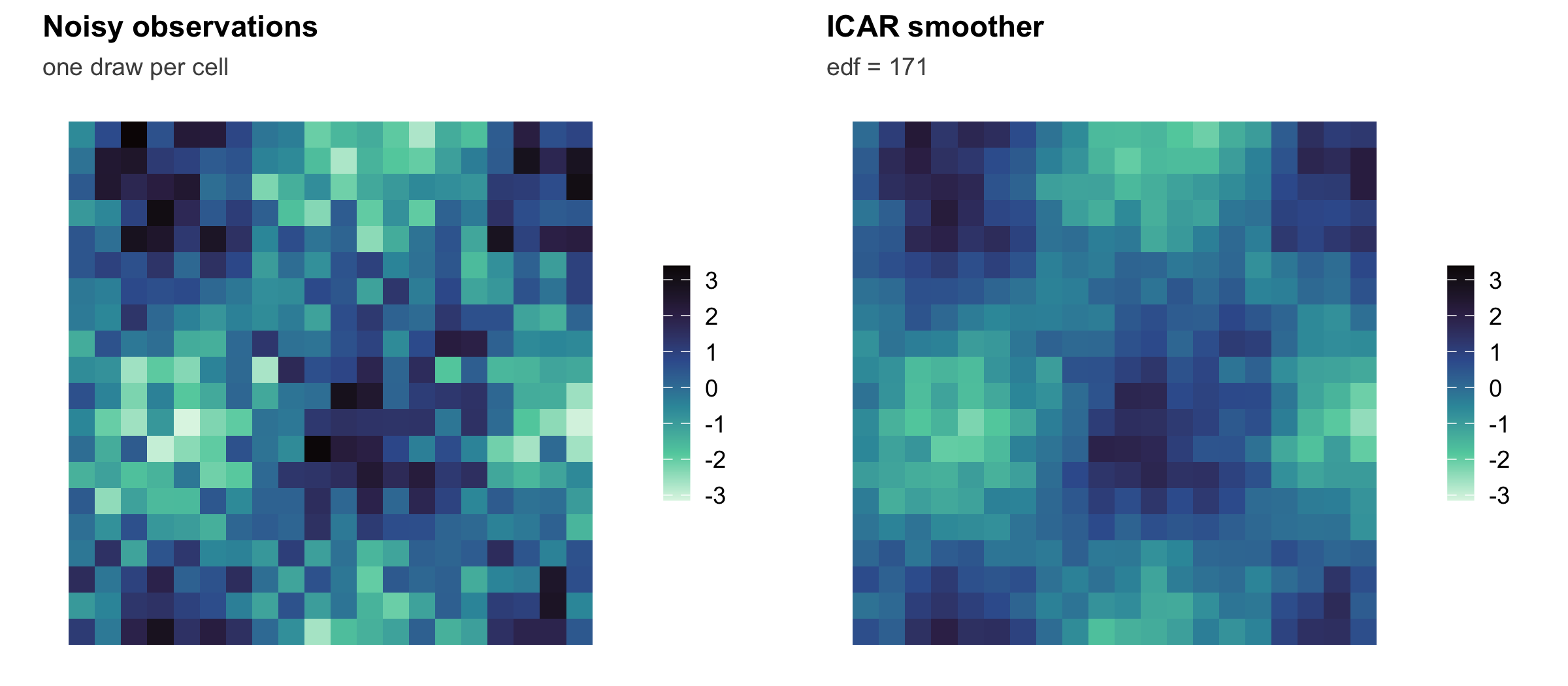
Push rho all the way to its boundary and the precision becomes D - A, the graph Laplacian. This is the intrinsic CAR (ICAR): an improper distribution (it has no overall level, hence the usual sum-to-zero constraint) that penalises differences between neighbours. It is the most widely used spatial random effect in ecology and epidemiology, because as a smoother it borrows strength across the map. To see it work, we take a noisy signal, one observation per cell, and recover the underlying smooth field.

set.seed(4232)
truef <- as.numeric(scale(1.4 * sin(pi * coords$col / 8) * cos(pi * coords$row / 9)))
yn    <- truef + rnorm(n, 0, 1.0)          # noisy observation per cell
R_icar <- D - A                            # intrinsic precision (graph Laplacian)
# GMRF smoother S = (I + kappa R)^{-1}; choose kappa by generalised cross-validation
gcv <- function(kappa) {
  S <- solve(diag(n) + kappa * R_icar); fit <- S %*% yn
  n * sum((yn - fit)^2) / (n - sum(diag(S)))^2
}
ks <- 10^seq(-2, 2, length = 40); k_opt <- ks[which.min(sapply(ks, gcv))]
Sopt   <- solve(diag(n) + k_opt * R_icar)
fit_ic <- as.numeric(Sopt %*% yn)
icar_kappa    <- k_opt
icar_edf      <- sum(diag(Sopt))
icar_rmse_raw <- sqrt(mean((yn - truef)^2))
icar_rmse_sm  <- sqrt(mean((fit_ic - truef)^2))
round(c(kappa = icar_kappa, edf = icar_edf,
        rmse_raw = icar_rmse_raw, rmse_smooth = icar_rmse_sm), 3)

      kappa         edf    rmse_raw rmse_smooth 
      0.438     171.406       0.894       0.422 

Cross-validation settles on a smoother with about 171 effective degrees of freedom out of 400 cells. It cuts the root mean squared error against the truth from 0.89 for the raw observations to 0.42, roughly halving it, simply by letting each cell learn from its neighbours. This borrowing of strength is exactly what an ICAR random effect does inside a larger model.

Noisy per-cell observations (left) and the same cells after the intrinsic CAR smoother (right), drawn on a common colour scale.

What to carry forward

A CAR model is built from local conditional rules and summarised by a sparse precision matrix D - rho A. It is the natural spatial term for hierarchical and generalised linear mixed models, where the conditional form slots neatly into the wider structure. Three points are worth remembering. The autocorrelation parameter depends on the weights convention, so it is not portable between software. A CAR and a SAR on the same neighbourhood imply genuinely different covariances, and the choice between them is substantive, not cosmetic. And the intrinsic CAR, the boundary case, is less a model of correlation than a smoother, penalising neighbour differences to pool information.

That smoothing power comes with a hidden cost. When the spatial random effect is flexible enough to mimic a spatially structured covariate, it can quietly absorb that covariate’s effect. This is spatial confounding, and checking a spatial regression takes it apart in detail.

References

Besag J 1974 Journal of the Royal Statistical Society: Series B 36(2):192-225 (10.1111/j.2517-6161.1974.tb00999.x)

Dormann CF, McPherson JM, Araujo MB, Bivand R, Bolliger J, Carl G, et al. 2007 Ecography 30(5):609-628 (10.1111/j.2007.0906-7590.05171.x)

Ver Hoef JM, Peterson EE, Hooten MB, Hanks EM, Fortin M-J 2018 Ecological Monographs 88(1):36-59 (10.1002/ecm.1283)

Related tutorials

• Spatial lag and spatial error models (SAR) build areal dependence from a single simultaneous equation.
• Moran eigenvector spatial filtering offers a third route that fits inside a generalised linear model.
• Checking a spatial regression compares CAR, SAR and filtering and exposes spatial confounding.
• Generalised least squares for spatial correlation covers the continuous-distance analogue.

Reproducibility

• Code last run: 2026-10-15
• R version 4.5.3 (2026-03-11), aarch64-apple-darwin20
• Packages: ggplot2 4.0.3