library(ggplot2)

te_pal <- list(forest = "#275139", green = "#2f8f63", sage = "#93a87f",
               clay = "#b5534e", gold = "#cda23f", line = "#dad9ca",
               ink = "#16241d", paper = "#f5f4ee")

theme_te <- function() {
  theme_minimal(base_size = 12) +
    theme(panel.grid.minor = element_blank(),
          panel.grid.major = element_line(colour = "#e7e6dc"),
          plot.background = element_rect(fill = "#f5f4ee", colour = NA),
          panel.background = element_rect(fill = "#f5f4ee", colour = NA),
          plot.title = element_text(face = "bold", colour = te_pal$ink),
          axis.title = element_text(colour = "#2c3a31"),
          axis.text = element_text(colour = "#2c3a31"))
}The variogram and the GP kernel
R
spatial
geostatistics
Bayesian statistics
ecology tutorial
The geostatistical variogram and the Gaussian process kernel are one object in two notations. The dictionary, a numerical check, and where the estimators part.
An ecologist who learned spatial statistics from a soil science course fits a variogram, reads off a nugget, a partial sill and a range, and hands those three numbers to a kriging routine. An ecologist who learned it from a machine learning course writes down a kernel, optimises a noise variance, a signal variance and a length-scale by marginal likelihood, and takes the posterior mean. The two produce the same map. Neither literature says so in a way that lets you convert one set of numbers into the other, so people fluent in one often cannot read a paper using the other.
This blog has half of the connection already. The Gaussian process regression post says three separate times that the same machinery taken onto a map is kriging, and it is right, but it says it in a single clause each time and never measures it. The kriging post, which is where the variogram vocabulary lives, does not contain the words “Gaussian process” or “kernel” anywhere. The two posts do not even use the same correlation function: one is exponential and the other squared exponential. So the claim has been asserted on this site and never cashed. This post cashes it. It writes out the dictionary term by term, verifies the correspondence with numbers, and then finds the place where the equivalence stops holding, which is not in the model at all but in how the three numbers get estimated.
The setting is a forest reserve twenty kilometres on a side where canopy openness has been measured at scattered plots, and the question is a map of openness at places nobody visited. The data is synthetic, generated from a covariance function we choose, so every claim about recovering a parameter can be checked against the value that produced the field. Some plots sit in short-distance clusters, the standard trick for getting information about the nugget: without pairs a few hundred metres apart, the shortest sampled gap is a kilometre and the nugget is an extrapolation. Three things get measured. The predictor from the two traditions agrees to the last bit of double precision, while the prediction variance differs by exactly one term whose identity turns out to be informative. The estimators do not agree, and the gap is large enough to matter in one place. And the mistake this dictionary prevents, confusing the range parameter with the distance at which correlation dies, costs almost nothing in the map and a great deal in the error bars.
Two vocabularies, one covariance function
Write the measured value at location \(s\) as a constant mean plus a smooth spatial term plus independent measurement error,
\[Z(s) = \mu + f(s) + \varepsilon(s), \qquad f \sim \mathcal{GP}(0, k), \qquad \varepsilon(s) \sim N(0, \sigma_n^2)\]
with \(k(h) = \sigma_f^2 \rho(h)\) a covariance depending only on the separation \(h\). That is the Gaussian process statement of the model. The geostatistical statement is that \(Z\) is second-order stationary with covariance \(C(h)\), and it works with the semivariogram
\[\gamma(h) = \tfrac{1}{2}\,\mathbb{E}\big[(Z(s+h) - Z(s))^2\big].\]
Expand the square. The expectation of \((Z(s+h) - Z(s))^2\) is \(\mathbb{E}Z(s+h)^2 + \mathbb{E}Z(s)^2 - 2\,\mathbb{E}[Z(s)Z(s+h)]\), and under stationarity the first two terms are both \(C(0)\) and the last is \(C(h)\). Halving gives the whole relationship:
\[\gamma(h) = C(0) - C(h).\]
The semivariogram is the covariance function turned upside down about \(C(0)/2\). Nothing else is going on. Substituting the model above, \(C(0) = \sigma_f^2 + \sigma_n^2\), and for any \(h > 0\) the measurement errors at two distinct locations are independent so \(C(h) = \sigma_f^2 \rho(h)\). Therefore
\[\gamma(h) = \sigma_n^2 + \sigma_f^2\big(1 - \rho(h)\big), \quad h > 0, \qquad \gamma(0) = 0,\]
which is exactly the nugget-plus-structure shape a variogram plot shows. Reading the three geostatistical quantities off that expression gives the dictionary.
| geostatistics | Gaussian processes | this post |
|---|---|---|
| nugget | noise variance | \(\sigma_n^2\) |
| partial sill | signal variance | \(\sigma_f^2\) |
| sill | prior variance of an observation | \(\sigma_f^2 + \sigma_n^2\) |
| range parameter | length-scale | \(\ell\) |
| practical range | no standard name | \(\approx 3\ell\) |
| semivariogram \(\gamma(h)\) | \(C(0) - k(h)\) for \(h>0\) | |
| simple kriging | GP posterior mean, mean known | |
| ordinary kriging | GP posterior mean, constant mean profiled out |
The practical range row causes the most trouble. For the exponential model \(\rho(h) =
\exp(-h/\ell)\) the correlation never reaches zero, so geostatistics reports the distance at which it has fallen to five per cent while machine learning reports \(\ell\) itself; the two differ by a fixed factor the chunk below prints. Software does not agree on which to display, gstat giving \(\ell\) in the range column of a fitted vgm object while plotting a curve that flattens at about three times that, and papers routinely quote the flattening distance as “the range”. Take a published range into a kernel and you may be off by a factor of three.
cov_exp <- function(h, nugget, psill, ell) {
  ifelse(h == 0, nugget + psill, psill * exp(-h / ell))
}
vgm_exp <- function(h, nugget, psill, ell) {
  ifelse(h == 0, 0, nugget + psill * (1 - exp(-h / ell)))
}

nugget_true <- 0.8
psill_true <- 4.0
ell_true <- 2.5
mu_true <- 18
sill_true <- nugget_true + psill_true
prac_fac <- -log(0.05)

h_chk <- c(0, seq(0.02, 20, length.out = 2000))
gap <- cov_exp(h_chk, nugget_true, psill_true, ell_true) +
  vgm_exp(h_chk, nugget_true, psill_true, ell_true) - sill_true

print(c(nugget = nugget_true, partial_sill = psill_true, sill = sill_true,
        length_scale_km = ell_true, mean_openness = mu_true))
nugget partial_sill sill length_scale_km mean_openness
0.8 4.0 4.8 2.5 18.0 print(signif(c(max_abs_gap_C_plus_gamma_minus_sill = max(abs(gap))), 3))max_abs_gap_C_plus_gamma_minus_sill
8.88e-16 print(round(c(practical_range_factor = prac_fac,
practical_range_km = prac_fac * ell_true,
correlation_at_one_length_scale = exp(-1),
correlation_at_practical_range = exp(-prac_fac)), 4)) practical_range_factor practical_range_km
2.9957 7.4893
correlation_at_one_length_scale correlation_at_practical_range
0.3679 0.0500 Across 2001 separations from zero to 20 kilometres the identity \(C(h) + \gamma(h) = C(0)\) holds to 8.88e-16, which is floating point and not statistics. The practical range factor is 2.9957, so with a length-scale of 2.5 kilometres the curve flattens visibly at 7.4893 kilometres. At one length-scale the correlation is still 0.3679.
Checking the dictionary on a simulated field
An identity between two formulas is cheap. The claim worth checking is that the estimator a geostatistician computes from data, the binned method-of-moments semivariance, has \(C(0) - C(h)\) as its expectation. Simulate a field from the kernel, compute
\[\hat\gamma(h_k) = \frac{1}{2 |N_k|} \sum_{(i,j) \in N_k} \big(z_i - z_j\big)^2\]
over the pairs whose separation falls in bin \(k\), average over many realisations of the field at the same plot locations, and compare bin by bin with the theoretical value. The right target is the mean of \(\gamma\) over the separations actually in the bin, not \(\gamma\) at the mean separation, because the bin has width and the curve is not straight across it.
set.seed(20260801)
side_km <- 20
n_open <- 96
n_clus <- 24
par_id <- sample.int(n_open, n_clus, replace = TRUE)
ang <- runif(n_clus, 0, 2 * pi)
rad <- runif(n_clus, 0.05, 0.5)
xy_open <- cbind(runif(n_open, 0, side_km), runif(n_open, 0, side_km))
xy <- rbind(xy_open,
            cbind(pmin(pmax(xy_open[par_id, 1] + rad * cos(ang), 0), side_km),
                  pmin(pmax(xy_open[par_id, 2] + rad * sin(ang), 0), side_km)))
n_pt <- nrow(xy)
D <- as.matrix(dist(xy))
iu <- upper.tri(D)
h_all <- D[iu]

Lchol <- chol(psill_true * exp(-D / ell_true) + 1e-9 * diag(n_pt))
sim_field <- function() {
  as.vector(mu_true + crossprod(Lchol, rnorm(n_pt)) +
              rnorm(n_pt, 0, sqrt(nugget_true)))
}

cutoff_km <- 10
n_bin <- 15
brk <- seq(0, cutoff_km, length.out = n_bin + 1)
bin_id <- cut(h_all, brk, labels = FALSE)
keep <- !is.na(bin_id)
bin_k <- bin_id[keep]
h_mid <- as.vector(tapply(h_all[keep], bin_k, mean))
np_bin <- as.vector(tapply(h_all[keep], bin_k, length))

emp_gamma <- function(z) {
  d2 <- 0.5 * (outer(z, z, "-")^2)[iu][keep]
  as.vector(tapply(d2, bin_k, mean))
}

print(round(c(plots = n_pt, open_plots = n_open, cluster_plots = n_clus,
              block_side_km = side_km, shortest_pair_km = min(h_all),
              pairs_total = length(h_all), pairs_under_1km = sum(h_all < 1),
              cutoff_km = cutoff_km, bins = n_bin, pairs_used = sum(np_bin)), 4))
plots open_plots cluster_plots block_side_km
120.0000 96.0000 24.0000 20.0000
shortest_pair_km pairs_total pairs_under_1km cutoff_km
0.0622 7140.0000 64.0000 10.0000
bins pairs_used
15.0000 3512.0000 120 plots give 7140 pairs, of which 3512 fall inside the 10 kilometre cutoff and get binned. The clusters buy 64 pairs closer than a kilometre, the shortest being 0.0622 kilometres.
set.seed(20260802)
n_rep1 <- 1500
acc <- matrix(0, n_rep1, n_bin)
for (r in seq_len(n_rep1)) acc[r, ] <- emp_gamma(sim_field())
gbar <- colMeans(acc)
g_se <- apply(acc, 2, sd) / sqrt(n_rep1)
g_exact <- as.vector(tapply(vgm_exp(h_all[keep], nugget_true, psill_true,
                                    ell_true), bin_k, mean))
g_mid <- vgm_exp(h_mid, nugget_true, psill_true, ell_true)
z_dev <- (gbar - g_exact) / g_se
print(round(data.frame(h_km = h_mid, pairs = np_bin, empirical = gbar,
                       theory = g_exact, se = g_se, z = z_dev), 4))
h_km pairs empirical theory se z
1 0.3549 39 1.3222 1.3208 0.0088 0.1650
2 1.0458 62 2.1630 2.1607 0.0121 0.1900
3 1.6773 112 2.7695 2.7493 0.0143 1.4115
4 2.3382 151 3.2099 3.2256 0.0163 -0.9645
5 3.0117 193 3.6252 3.5972 0.0185 1.5147
6 3.6693 221 3.9011 3.8752 0.0210 1.2318
7 4.3240 287 4.1352 4.0883 0.0231 2.0331
8 4.9983 283 4.3009 4.2568 0.0253 1.7421
9 5.6807 275 4.4459 4.3864 0.0277 2.1456
10 6.3493 298 4.5415 4.4835 0.0289 2.0068
11 6.9813 321 4.5947 4.5541 0.0293 1.3856
12 7.6870 324 4.6591 4.6147 0.0315 1.4121
13 8.3051 302 4.6844 4.6553 0.0312 0.9302
14 9.0086 321 4.7277 4.6908 0.0320 1.1552
15 9.6670 323 4.7455 4.7160 0.0322 0.9151print(round(c(realisations = n_rep1,
max_abs_deviation = max(abs(gbar - g_exact)),
max_relative_deviation = max(abs(gbar - g_exact) / g_exact),
max_abs_z = max(abs(z_dev)), mean_z = mean(z_dev)), 4)) realisations max_abs_deviation max_relative_deviation
1500.0000 0.0595 0.0136
max_abs_z mean_z
2.1456 1.1516 print(round(c(mean_sep_target_max_abs_dev = max(abs(gbar - g_mid))), 4))mean_sep_target_max_abs_dev
0.0582 mid_gap <- vapply(c(5, 10, 15, 25, 40), function(nb) {
bkk <- cut(h_all, seq(0, cutoff_km, length.out = nb + 1), labels = FALSE)
gt <- vgm_exp(h_all, nugget_true, psill_true, ell_true)
hm <- tapply(h_all, bkk, mean)[1]
tapply(gt, bkk, mean)[1] - vgm_exp(hm, nugget_true, psill_true, ell_true)
}, numeric(1))
names(mid_gap) <- paste0("first_bin_gap_", c(5, 10, 15, 25, 40), "_bins")
print(round(mid_gap, 4)) first_bin_gap_5_bins first_bin_gap_10_bins first_bin_gap_15_bins
-0.0588 -0.0225 -0.0086
first_bin_gap_25_bins first_bin_gap_40_bins
-0.0025 -0.0010 Averaged over 1500 realisations at the same 120 plots, the binned semivariance sits on the curve \(C(0) - C(h)\) to within 0.0595 in the worst bin, 1.36 per cent of the value there, and the largest discrepancy over the 15 bins is 2.15 Monte Carlo standard errors. Read that column with the bins in mind: they are not 15 independent tests, since every bin comes from the same fields, so the deviations move together and the whole set is displaced upward by 1.15 standard errors. One correlated quantity two standard errors from zero is an ordinary draw. The method-of-moments variogram estimates the kernel, in the sense that a sample mean estimates a population mean.
One detail comes back later. A fitted variogram compares the binned average to the model evaluated at a single distance, the mean separation of the pairs in it, which is what gstat uses and what the fits below use, and those two stop agreeing once the bins get wide. In the first bin the within-bin average of \(\gamma\) sits -0.0588 from the value at that mean separation at five bins and -0.001 at forty, a factor of 61. The sign is negative, so under coarse binning the first point looks lower than the model says it should, and something has to absorb that.
h_plot <- seq(0.02, 12, length.out = 400)
mirror <- rbind(
  data.frame(h = h_plot, y = cov_exp(h_plot, nugget_true, psill_true, ell_true),
             fn = "covariance C(h), the GP kernel"),
  data.frame(h = h_plot, y = vgm_exp(h_plot, nugget_true, psill_true, ell_true),
             fn = "semivariogram gamma(h)"))
pts <- data.frame(h = h_mid, y = gbar)

ggplot(mirror, aes(h, y, colour = fn)) +
  geom_hline(yintercept = sill_true / 2, linetype = "22",
             colour = "#9aa295") +
  geom_vline(xintercept = prac_fac * ell_true, linetype = "31",
             colour = "#9aa295") +
  geom_line(linewidth = 0.9) +
  geom_point(data = pts, aes(h, y), inherit.aes = FALSE,
             colour = te_pal$sage, size = 2) +
  annotate("text", x = 11.6, y = sill_true / 2 + 0.16, hjust = 1,
           label = "half the sill", size = 3.1, colour = "#6d7568") +
  annotate("text", x = prac_fac * ell_true + 0.2, y = 0.35, hjust = 0,
           label = "practical range", size = 3.1, colour = "#6d7568") +
  scale_colour_manual(values = c(te_pal$forest, te_pal$clay), name = NULL) +
  labs(x = "separation h (km)", y = "value",
       title = "One function, drawn both ways up") +
  theme_te() +
  theme(legend.position = "bottom", plot.margin = margin(8, 14, 4, 8))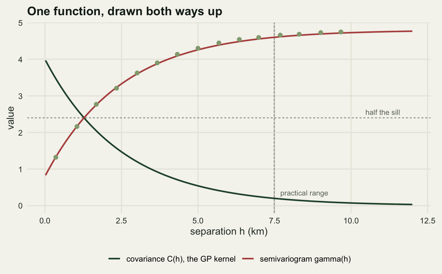
The dotted vertical line marks the practical range at 7.49 kilometres, where the red curve has closed 95 per cent of its climb from nugget to sill. At the length-scale itself, 2.5 kilometres, the green curve has lost only 63.2 per cent of its height. Reading a range off a plot by eye gives you the dotted line, not the length-scale.
The predictor is the same object written twice
The dictionary would be a curiosity if the two traditions then did different arithmetic with the three numbers. They do not. The geostatistician builds the matrix of semivariances between plots, converts it to covariances by subtracting from the sill, and solves the kriging system; the GP user builds the kernel matrix directly, adds the noise variance to its diagonal, and takes a posterior mean. The two routes below are the same linear algebra: one through solve on a matrix assembled from vgm_exp, the other through a Cholesky factor of one assembled from exp(-D/ell).
set.seed(20260803)
z_obs <- sim_field()

gr <- expand.grid(x = seq(0.5, 19.5, by = 1), y = seq(0.5, 19.5, by = 1))
n_gr <- nrow(gr)
D_star <- as.matrix(dist(rbind(xy, as.matrix(gr))))[1:n_pt, n_pt + (1:n_gr)]

# route A: variogram, simple kriging
Gam <- vgm_exp(D, nugget_true, psill_true, ell_true)
Gam_s <- vgm_exp(D_star, nugget_true, psill_true, ell_true)
C_kr <- sill_true - Gam
c_kr <- sill_true - Gam_s
w_kr <- solve(C_kr, c_kr)
pred_kr <- mu_true + as.vector(crossprod(w_kr, z_obs - mu_true))
var_kr <- sill_true - colSums(c_kr * w_kr)

# route B: kernel, GP posterior
K <- psill_true * exp(-D / ell_true) + nugget_true * diag(n_pt)
K_s <- psill_true * exp(-D_star / ell_true)
Rc <- chol(K)
alpha <- backsolve(Rc, backsolve(Rc, z_obs - mu_true, transpose = TRUE))
pred_gp <- mu_true + as.vector(crossprod(K_s, alpha))
Vs <- backsolve(Rc, K_s, transpose = TRUE)
var_gp <- psill_true - colSums(Vs^2)

d_pred <- max(abs(pred_kr - pred_gp))
d_var <- var_kr - var_gp
print(round(c(grid_nodes = n_gr, observed_min = min(z_obs),
              observed_max = max(z_obs), predicted_min = min(pred_gp),
              predicted_max = max(pred_gp), kriging_var_min = min(var_kr),
              kriging_var_max = max(var_kr), gp_var_min = min(var_gp),
              gp_var_max = max(var_gp)), 4))
grid_nodes observed_min observed_max predicted_min predicted_max
400.0000 14.3123 23.8991 14.9610 21.7933
kriging_var_min kriging_var_max gp_var_min gp_var_max
1.4086 4.2865 0.6086 3.4865 print(signif(c(max_abs_prediction_gap = d_pred,
max_relative_gap = max(abs(pred_kr - pred_gp) / abs(pred_gp)),
sd_of_variance_gap = sd(d_var)), 3))max_abs_prediction_gap max_relative_gap sd_of_variance_gap
1.07e-14 6.53e-16 1.49e-15 print(round(c(mean_variance_gap = mean(d_var), nugget = nugget_true), 6))mean_variance_gap nugget
0.8 0.8 On a grid of 400 nodes the two predictors differ by at most 1.07e-14 in absolute terms and 6.53e-16 in relative terms, roughly one part in \(10^{15}\): not agreement within tolerance but the same number computed twice with different rounding. Simple kriging and the GP posterior mean are one formula.
The variances are where something real shows up. The kriging variance runs from 1.4086 to 4.2865, the GP posterior variance from 0.6086 to 3.4865, and the difference is 0.8 at every one of the 400 nodes, with a standard deviation across nodes of 1.49e-15. It is the nugget, exactly.
That gap is a difference in the question, not a discrepancy. The kriging variance as usually written is for the prediction error of a new measurement, including that measurement’s own nugget; the GP posterior variance is for the underlying function \(f\), with the noise left out. Add \(\sigma_n^2\) back and you have the kriging variance, which is what a GP library returns when you ask for the predictive distribution of \(y_*\) rather than \(f_*\). Confusing them misstates the interval half-width by the square root of their ratio, which across the 400 nodes runs from 1.109 to 1.521: worst where plots are dense and the posterior variance is small, the part of the map you trust most.
If you use gstat, the call below produces the same surface. It is not run here (the package is absent from the render machine) and is included so the argument names line up with the dictionary: psill is the signal variance, nugget the noise variance, range the length-scale.
library(gstat)
library(sf)
pts_sf <- st_as_sf(data.frame(xy, z = z_obs), coords = c("V1", "V2"))
mod <- vgm(psill = psill_true, model = "Exp", range = ell_true,
           nugget = nugget_true)
kr <- krige(z ~ 1, pts_sf, newdata = st_as_sf(gr, coords = c("x", "y")),
            model = mod)
Where the traditions part: the estimator
Everything so far assumed the three numbers were handed to us. They are not, and here is where the two literatures genuinely diverge. The geostatistical route reduces the data to a binned empirical variogram and fits the model curve to those points by weighted least squares, with weights proportional to the pair count and inversely to the squared model value (Cressie 1985):
\[\hat\theta_{\text{WLS}} = \arg\min_\theta \sum_k |N_k| \left(\frac{\hat\gamma_k}{\gamma(h_k;\theta)} - 1\right)^2.\]
The Gaussian process route never bins anything: it writes the multivariate normal likelihood of the whole vector, profiles the constant mean out by generalised least squares, and maximises
\[-2\log L(\theta) = \log|C_\theta| + (z - \hat\mu)^\top C_\theta^{-1} (z - \hat\mu) + n \log 2\pi.\]
Both are written out below in base R. The WLS objective touches the data once, through the 15 binned averages, and never again; the likelihood touches all 7260 distinct entries of the covariance matrix at every evaluation and needs a Cholesky factorisation each time.
cnt <- new.env()
cnt$wls <- cnt$ml <- cnt$chol <- 0L
lo_par <- log(c(1e-3, 1e-3, 0.05))
hi_par <- log(c(20, 100, cutoff_km))

wls_fit <- function(gh, hm, np, start) {
  obj <- function(p) {
    th <- exp(p)
    cnt$wls <- cnt$wls + 1L
    g <- th[1] + th[2] * (1 - exp(-hm / th[3]))
    sum(np * (gh / g - 1)^2)
  }
  o <- optim(log(start), obj, method = "L-BFGS-B", lower = lo_par,
             upper = hi_par, control = list(factr = 1e2))
  exp(o$par)
}

ml_fit <- function(z, Dm, start) {
  n <- length(z)
  one <- rep(1, n)
  nll <- function(p) {
    th <- exp(p)
    cnt$ml <- cnt$ml + 1L
    Cm <- th[2] * exp(-Dm / th[3])
    diag(Cm) <- th[1] + th[2]
    Rr <- tryCatch(chol(Cm), error = function(e) NULL)
    if (is.null(Rr)) return(1e10)
    cnt$chol <- cnt$chol + 1L
    A <- backsolve(Rr, backsolve(Rr, cbind(one, z), transpose = TRUE))
    mu <- sum(A[, 2]) / sum(A[, 1])
    r <- z - mu
    Cir <- backsolve(Rr, backsolve(Rr, r, transpose = TRUE))
    sum(log(diag(Rr))) + 0.5 * sum(r * Cir) + 0.5 * n * log(2 * pi)
  }
  o <- optim(log(start), nll, method = "L-BFGS-B", lower = lo_par,
             upper = hi_par, control = list(factr = 1e2))
  exp(o$par)
}

st_par <- c(0.5, 3, 2)
p_wls <- wls_fit(emp_gamma(z_obs), h_mid, np_bin, st_par)
p_ml <- ml_fit(z_obs, D, st_par)

one_tab <- rbind(truth = c(nugget_true, psill_true, ell_true),
                 wls = p_wls, ml = p_ml)
colnames(one_tab) <- c("nugget", "partial_sill", "length_scale")
print(round(one_tab, 4))
nugget partial_sill length_scale
truth 0.8000 4.0000 2.5000
wls 0.8914 4.1769 6.3736
ml 0.9585 2.7837 4.3904print(round(c(wls_practical_range = prac_fac * p_wls[3],
ml_practical_range = prac_fac * p_ml[3],
wls_sill = sum(p_wls[1:2]), ml_sill = sum(p_ml[1:2])), 4))wls_practical_range ml_practical_range wls_sill ml_sill
19.0935 13.1526 5.0682 3.7423 Run on the field already used for the prediction check, the two disagree in a way that would change what you wrote in a paper. WLS returns a length-scale of 6.3736 kilometres, maximum likelihood 4.3904, against a truth of 2.5; as practical ranges, 19.1 kilometres against 13.2, the first nearly the width of the whole reserve. The nuggets are close, 0.8914 and 0.9585 against 0.8, and the partial sills 4.1769 and 2.7837 against 4. Both overshoot the length-scale here, which one draw of a random field is entitled to do, and one dataset says nothing about which estimator is better, so the next chunk repeats it.
n_rep <- 200
res <- matrix(NA_real_, n_rep, 6)
z_store <- vector("list", n_rep)
set.seed(20260805)
cnt$wls <- cnt$ml <- cnt$chol <- 0L
for (r in seq_len(n_rep)) {
  zz <- sim_field()
  z_store[[r]] <- zz
  res[r, 1:3] <- wls_fit(emp_gamma(zz), h_mid, np_bin, st_par)
  res[r, 4:6] <- ml_fit(zz, D, st_par)
}

tv <- c(nugget_true, psill_true, ell_true)
summ <- data.frame(
  truth = tv,
  wls_bias = colMeans(res[, 1:3]) - tv,
  ml_bias = colMeans(res[, 4:6]) - tv,
  wls_sd = apply(res[, 1:3], 2, sd),
  ml_sd = apply(res[, 4:6], 2, sd),
  wls_median = apply(res[, 1:3], 2, median),
  ml_median = apply(res[, 4:6], 2, median))
summ$sd_ratio <- summ$wls_sd / summ$ml_sd
summ$wls_rmse <- sqrt(colMeans((res[, 1:3] - rep(tv, each = n_rep))^2))
summ$ml_rmse <- sqrt(colMeans((res[, 4:6] - rep(tv, each = n_rep))^2))
summ$rmse_ratio <- summ$wls_rmse / summ$ml_rmse
rownames(summ) <- c("nugget", "partial_sill", "length_scale")
print(round(summ, 4))
truth wls_bias ml_bias wls_sd ml_sd wls_median ml_median sd_ratio
nugget 0.8 -0.0778 -0.0770 0.5062 0.3149 0.6553 0.7264 1.6074
partial_sill 4.0 0.3792 -0.2207 1.5733 0.9501 4.0844 3.6956 1.6559
length_scale 2.5 0.5826 -0.1187 2.3108 1.1696 2.2571 2.2016 1.9757
wls_rmse ml_rmse rmse_ratio
nugget 0.5109 0.3234 1.5796
partial_sill 1.6145 0.9731 1.6592
length_scale 2.3775 1.1727 2.0274wls_evals <- cnt$wls / n_rep
ml_evals <- cnt$ml / n_rep
chol_per_set <- cnt$chol / n_rep
n_bound_w <- sum(res[, 3] > cutoff_km - 1e-6)
n_bound_m <- sum(res[, 6] > cutoff_km - 1e-6)
print(c(datasets = n_rep, wls_length_scale_at_bound = n_bound_w,
ml_length_scale_at_bound = n_bound_m, upper_bound_km = cutoff_km)) datasets wls_length_scale_at_bound ml_length_scale_at_bound
200 11 1
upper_bound_km
10 par_lab <- c("nugget", "partial sill", "length-scale (km)")
samp <- data.frame(
value = as.vector(res),
parameter = factor(rep(rep(par_lab, each = n_rep), 2), levels = par_lab),
method = factor(rep(c("weighted least squares", "maximum likelihood"),
each = 3 * n_rep),
levels = c("maximum likelihood", "weighted least squares")))
truth_df <- data.frame(parameter = factor(par_lab, levels = par_lab), value = tv)
ggplot(samp, aes(method, value, fill = method)) +
geom_hline(data = truth_df, aes(yintercept = value), linetype = "22",
colour = "#6d7568") +
geom_boxplot(width = 0.55, outlier.size = 0.9, outlier.colour = "#6d7568",
colour = te_pal$ink, linewidth = 0.35) +
facet_wrap(~parameter, nrow = 1, scales = "free_y") +
scale_fill_manual(values = c(te_pal$green, te_pal$clay), name = NULL) +
scale_x_discrete(labels = c("ML", "WLS")) +
labs(x = NULL, y = "estimate",
title = "Same model, two ways of fitting it") +
theme_te() +
theme(legend.position = "bottom", plot.margin = margin(8, 14, 4, 8))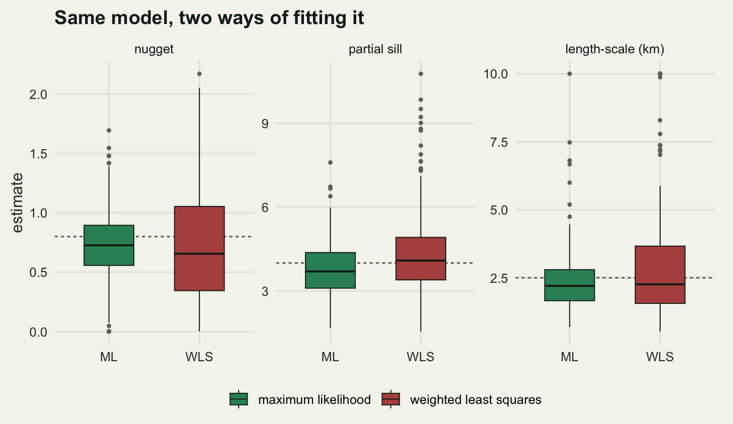
Over 200 datasets the biases are small next to the spread. Maximum likelihood is off by -0.077 on the nugget, -0.2207 on the partial sill and -0.1187 on the length-scale; weighted least squares by -0.0778, 0.3792 and 0.5826. Both pull the nugget low by nearly the same amount. The one that looks lopsided, the weighted least squares length-scale at 23 per cent of the truth, is mostly the upper tail rather than a shift of the bulk: the medians are 2.2571 and 2.2016, and the runs doing the lifting are the ones at the bound two paragraphs below.
The spread is where they separate. The ratio of standard deviations, WLS over ML, is 1.6074 on the nugget, 1.6559 on the partial sill and 1.9757 on the length-scale, and in root mean squared error the length-scale ratio is 2.0274. Fitting the binned variogram instead of the likelihood costs the equivalent of shrinking the survey, and costs most on the parameter people quote in papers.
The tail is worse than the standard deviation suggests. On 11 of the 200 datasets the WLS length-scale ran into the upper bound of 10 kilometres, the variogram cutoff and half the width of the block; maximum likelihood hit it on 1 of them. On those datasets the binned points fail to flatten inside the cutoff, so the fitted curve keeps climbing and the partial sill and length-scale run off together, only their ratio pinned down by a curve that never levels. The folk remedy is to change the cutoff or the bins and try again, which is the next section.
The binning is a modelling choice with a price
The empirical variogram is not the data but a summary of it, and the summary depends on a choice, the number of bins, with no counterpart on the likelihood side. Sweep it and see how far the answer moves.
bin_grid <- c(5, 10, 15, 25, 40)
n_sweep <- 60
sw <- expand.grid(rep = seq_len(n_sweep), bins = bin_grid)
sw$nugget <- sw$psill <- sw$ell <- NA_real_

for (i in seq_len(nrow(sw))) {
  bid <- cut(h_all, seq(0, cutoff_km, length.out = sw$bins[i] + 1),
             labels = FALSE)
  kk <- !is.na(bid)
  bkk <- bid[kk]
  zz <- z_store[[sw$rep[i]]]
  gh <- as.vector(tapply(0.5 * (outer(zz, zz, "-")^2)[iu][kk], bkk, mean))
  sw[i, c("nugget", "psill", "ell")] <-
    wls_fit(gh, as.vector(tapply(h_all[kk], bkk, mean)),
            as.vector(tapply(h_all[kk], bkk, length)), st_par)
}

agg <- aggregate(cbind(nugget, psill, ell) ~ bins, sw, median)
agg$nugget_iqr <- aggregate(nugget ~ bins, sw, IQR)$nugget
agg$ell_iqr <- aggregate(ell ~ bins, sw, IQR)$ell
agg$ell_at_bound <- aggregate(ell ~ bins, sw,
                              function(v) mean(v > cutoff_km - 1e-6))$ell
print(round(agg, 4))
bins nugget psill ell nugget_iqr ell_iqr ell_at_bound
1 5 0.4980 4.3664 2.2051 1.3051 2.9926 0.0833
2 10 0.4289 4.3006 2.0077 0.8642 1.9334 0.0167
3 15 0.6050 4.2055 2.0813 0.6766 1.9173 0.0500
4 25 0.6882 4.0934 2.1097 0.5573 2.0779 0.0500
5 40 0.7242 4.0758 2.1016 0.5429 2.3137 0.0667wide_ell <- tapply(sw$ell, list(sw$rep, sw$bins), identity)
wide_nug <- tapply(sw$nugget, list(sw$rep, sw$bins), identity)
spread_ell <- apply(wide_ell, 1, function(v) max(v) - min(v))
spread_nug <- apply(wide_nug, 1, function(v) max(v) - min(v))
rel_ell <- median(spread_ell / apply(wide_ell, 1, median))
rel_nug <- median(spread_nug / apply(wide_nug, 1, median))
print(round(c(datasets_swept = n_sweep, bin_choices = length(bin_grid),
median_spread_nugget = median(spread_nug),
median_spread_length = median(spread_ell),
relative_spread_nugget = rel_nug,
relative_spread_length = rel_ell), 4)) datasets_swept bin_choices median_spread_nugget
60.0000 5.0000 0.5337
median_spread_length relative_spread_nugget relative_spread_length
0.3848 1.0744 0.2064 print(round(c(nugget_median_5_bins = agg$nugget[1],
nugget_median_40_bins = agg$nugget[5],
nugget_fold_change = agg$nugget[5] / agg$nugget[1],
spread_length_over_ml_sd = median(spread_ell) / summ$ml_sd[3],
spread_nugget_over_ml_sd = median(spread_nug) / summ$ml_sd[1]), 4)) nugget_median_5_bins nugget_median_40_bins nugget_fold_change
0.4980 0.7242 1.4541
spread_length_over_ml_sd spread_nugget_over_ml_sd
0.3290 1.6948 qs <- function(v) c(median(v), quantile(v, 0.25), quantile(v, 0.75))
q_lab <- c("nugget", "length-scale (km)")
band <- do.call(rbind, lapply(bin_grid, function(nb) {
s <- sw[sw$bins == nb, ]
data.frame(bins = nb, quantity = q_lab, rbind(qs(s$nugget), qs(s$ell)))
}))
names(band)[3:5] <- c("mid", "lo", "hi")
band$quantity <- factor(band$quantity, levels = q_lab)
ref <- data.frame(quantity = factor(q_lab, levels = q_lab),
value = c(nugget_true, ell_true))
ggplot(band, aes(bins, mid, colour = quantity, fill = quantity)) +
geom_hline(data = ref, aes(yintercept = value), linetype = "22",
colour = "#6d7568") +
geom_ribbon(aes(ymin = lo, ymax = hi), alpha = 0.22, colour = NA) +
geom_line(linewidth = 0.9) +
geom_point(size = 2.2) +
facet_wrap(~quantity, nrow = 1, scales = "free_y") +
scale_x_log10(breaks = bin_grid) +
scale_colour_manual(values = c(te_pal$forest, te_pal$clay)) +
scale_fill_manual(values = c(te_pal$forest, te_pal$clay)) +
labs(x = "number of variogram bins", y = "weighted least squares estimate",
title = "A knob the likelihood does not have") +
theme_te() +
theme(legend.position = "none", plot.margin = margin(8, 14, 4, 8))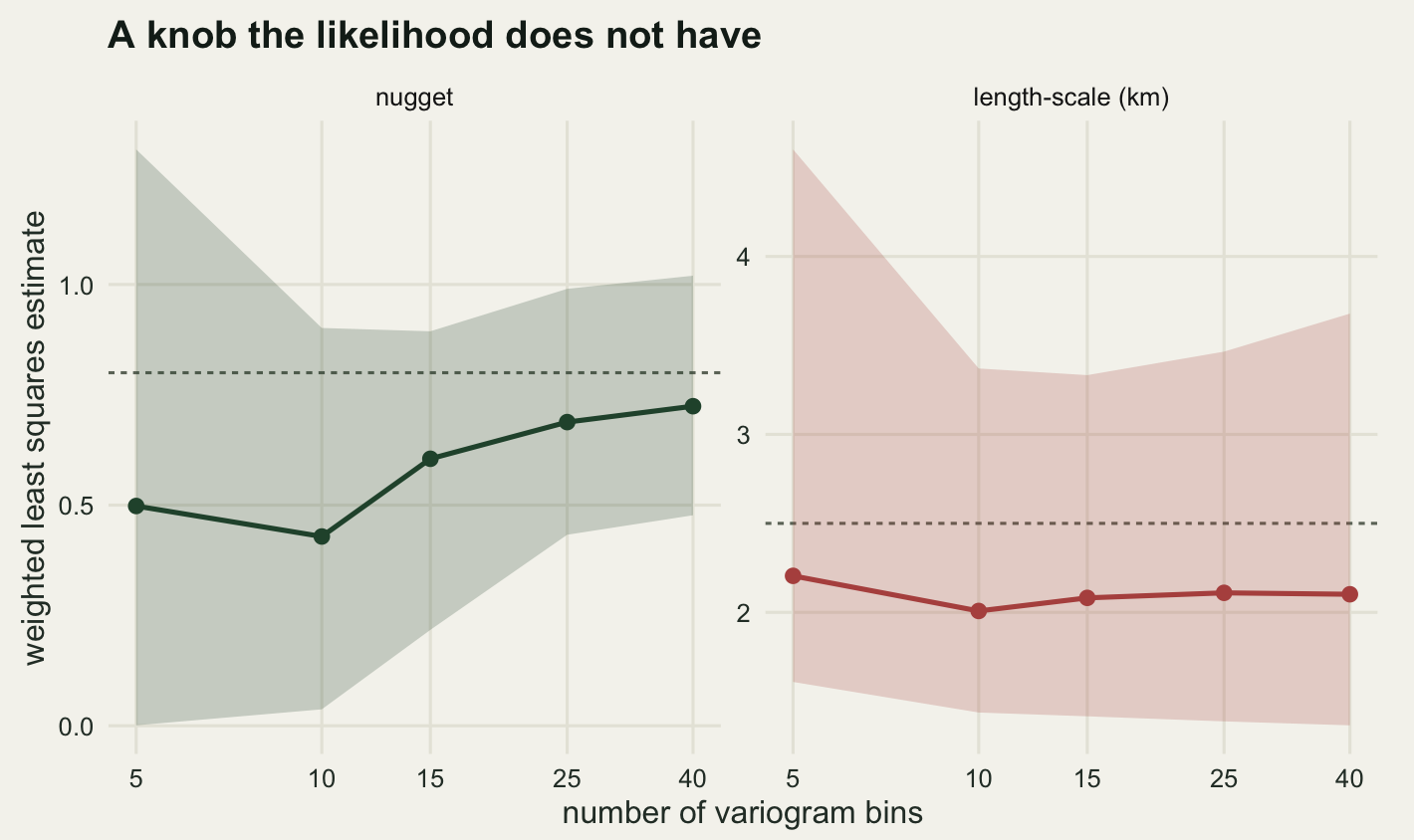
The nugget is the parameter the binning owns. Its median over the 60 datasets is 0.498 with 5 bins and 0.7242 with 40, a factor of 1.4541, against 0.8. Part of that is the mechanism measured earlier: at five bins the first binned average sits 0.0588 below the model evaluated at the mean separation in that bin, so the fit pulls the curve down near the origin and the nugget gives way. Only part, though, because that offset is 0.059 against a nugget shortfall of 0.302, roughly 19 per cent of the damage; the rest is the shape information lost when the first bin is two kilometres wide.
Within a single dataset, changing only the bin count moves the nugget by 0.5337 from best to worst case, 1.0744 of its own median: same data, same model, same estimator, and an answer that roughly doubles on a plotting choice. The length-scale is steadier in relative terms, moving 0.3848 kilometres or 0.2064 of its median.
Compare those to sampling noise. The likelihood estimator’s standard deviation over independent datasets was 0.3149 on the nugget and 1.1696 on the length-scale, so bin choice moves the nugget 1.6948 times the sampling standard deviation and the length-scale 0.329 times it. Those are best-to-worst ranges over five choices set against a standard deviation. Like for like, the nugget’s standard deviation across the five bin choices within one dataset is 0.2218, 0.44 of the sampling standard deviation of the same weighted least squares estimator: a plotting knob with no counterpart on the likelihood side costs about half of what a fresh survey costs. Maximum likelihood has no dial here at all.
The likelihood pays for that in arithmetic, and the honest way to state the cost is to count operations rather than seconds.
chol_flop <- function(n) n^3 / 3
ml_flops <- ml_evals * chol_flop(n_pt)
wls_flops <- n_pt * (n_pt - 1) / 2 + wls_evals * n_bin
print(round(c(datasets = n_rep, wls_objective_evals = wls_evals,
              ml_likelihood_evals = ml_evals,
              cholesky_factorisations = chol_per_set, matrix_size = n_pt), 2))
datasets wls_objective_evals ml_likelihood_evals
200.00 317.94 122.78
cholesky_factorisations matrix_size
122.78 120.00 print(signif(c(ml_flops_per_dataset = ml_flops,
wls_flops_per_dataset = wls_flops,
flop_ratio = ml_flops / wls_flops,
cholesky_flops_n1000 = chol_flop(1000),
cholesky_flops_n5000 = chol_flop(5000),
growth_120_to_5000 = chol_flop(5000) / chol_flop(n_pt),
ml_flops_if_n_5000 = ml_evals * chol_flop(5000)), 4)) ml_flops_per_dataset wls_flops_per_dataset flop_ratio
7.072e+07 1.191e+04 5.938e+03
cholesky_flops_n1000 cholesky_flops_n5000 growth_120_to_5000
3.333e+08 4.167e+10 7.234e+04
ml_flops_if_n_5000
5.116e+12 Per dataset the WLS fit took 317.9 objective evaluations, each 15 arithmetic operations on the binned summary, plus one pass over the 7140 pairs to build it. The likelihood fit took 122.8 evaluations, each a Cholesky factorisation of a 120 by 120 matrix, 122.78 in total: a flop ratio at this size of about 6000 to one. Both evaluation counts belong to the optimiser and will come out a little differently on another version of R; the cost of one evaluation will not.
That ratio is not a constant. The Cholesky is cubic, so going from 120 plots to five thousand multiplies the per-evaluation cost by 72340, to 4.17e+10 floating point operations for a single evaluation of the likelihood. A fit that takes 100 or so of them lands around 4e+12 operations in total, while the WLS side grows only with the number of pairs, quadratically, and the fit itself does not grow at all because the bins stay fixed. At a hundred plots the choice is free and you should take the likelihood. At five thousand it is a real decision, and the binned variogram survives at sizes where the dense likelihood does not. That, rather than tradition, is why geostatistics kept the two-stage procedure.
What the difference does to a map
Parameters are not the product. The map is, and a prediction interval on the map. Cross-validate: split the plots into ten folds and predict each held-out fold by ordinary kriging from the rest, once with the WLS parameters, once with the ML parameters, and once with the values that generated the field. The parameters are estimated on the full dataset in all three arms, so this measures what the parameter estimate does to prediction rather than the out-of-sample honesty of the fit; the truth as a third arm is what makes the other two readable.
A fourth arm is the mistake this post exists to prevent: the true partial sill and nugget, with the practical range plugged into the kernel as if it were the length-scale, an error of a factor of 2.996. That is what happens when a range is copied out of a paper, or read off a plot, and dropped into a covariance function.
ok_predict <- function(itr, ite, z, th) {
  Ctr <- th[2] * exp(-D[itr, itr, drop = FALSE] / th[3])
  diag(Ctr) <- th[1] + th[2]
  ktr <- th[2] * exp(-D[itr, ite, drop = FALSE] / th[3])
  Rr <- chol(Ctr)
  A <- backsolve(Rr, backsolve(Rr, cbind(rep(1, length(itr)), ktr),
                               transpose = TRUE))
  o1 <- sum(A[, 1])
  W <- A[, -1, drop = FALSE]
  Az <- backsolve(Rr, backsolve(Rr, z[itr], transpose = TRUE))
  mu <- sum(Az) / o1
  list(m = mu + as.vector(crossprod(ktr, Az - mu * A[, 1])),
       v = th[1] + th[2] - colSums(ktr * W) + (1 - colSums(W))^2 / o1)
}

mis_par <- c(nugget_true, psill_true, ell_true * prac_fac)
arms <- c("WLS", "ML", "truth", "range mislabelled")
n_cv <- 100
k_fold <- 10
zq <- qnorm(0.975)
set.seed(20260806)
fold <- sample(rep(seq_len(k_fold), length.out = n_pt))
cvo <- matrix(NA_real_, n_cv, 16)

for (r in seq_len(n_cv)) {
  zz <- z_store[[r]]
  ps <- list(res[r, 1:3], res[r, 4:6], tv, mis_par)
  for (j in seq_along(arms)) {
    e2 <- vv <- hit <- numeric(0)
    for (f in seq_len(k_fold)) {
      ite <- which(fold == f)
      pr <- ok_predict(which(fold != f), ite, zz, ps[[j]])
      e2 <- c(e2, (zz[ite] - pr$m)^2)
      vv <- c(vv, pr$v)
      hit <- c(hit, abs(zz[ite] - pr$m) <= zq * sqrt(pr$v))
    }
    cvo[r, j] <- sqrt(mean(e2))
    cvo[r, j + 4] <- mean(hit)
    cvo[r, j + 8] <- mean(e2 / vv)
    cvo[r, j + 12] <- mean(2 * zq * sqrt(vv))
  }
}

cv_tab <- data.frame(
  arm = arms,
  rmse = colMeans(cvo[, 1:4]),
  coverage = colMeans(cvo[, 5:8]),
  scaled_sq_resid = colMeans(cvo[, 9:12]),
  interval_width = colMeans(cvo[, 13:16]))
cv_tab$rmse_vs_truth <- cv_tab$rmse / cv_tab$rmse[3]
cv_tab$width_vs_truth <- cv_tab$interval_width / cv_tab$interval_width[3]
cv_tab$mean_abs_calib <- colMeans(abs(cvo[, 9:12] - 1))
print(round(cv_tab[, -1], 5))
rmse coverage scaled_sq_resid interval_width rmse_vs_truth width_vs_truth
1 1.56539 0.94433 1.02847 6.07133 0.99980 0.98948
2 1.55650 0.95033 1.00003 6.03191 0.99412 0.98305
3 1.56570 0.95125 0.98318 6.13590 1.00000 1.00000
4 1.58161 0.88025 1.57080 4.89856 1.01016 0.79834
mean_abs_calib
1 0.10065
2 0.03263
3 0.10911
4 0.57080print(cv_tab$arm)[1] "WLS" "ML" "truth"
[4] "range mislabelled"print(round(c(nominal = 0.95, datasets = n_cv, folds = k_fold,
sd_rmse_ratio_wls = sd(cvo[, 1] / cvo[, 3]),
sd_width_ratio_wls = sd(cvo[, 13] / cvo[, 15]),
sd_width_ratio_ml = sd(cvo[, 14] / cvo[, 15]),
worst_rmse_ratio_wls = max(cvo[, 1] / cvo[, 3])), 5)) nominal datasets folds
0.95000 100.00000 10.00000
sd_rmse_ratio_wls sd_width_ratio_wls sd_width_ratio_ml
0.01389 0.06751 0.05959
worst_rmse_ratio_wls
1.03398 sc <- data.frame(
rmse_ratio = c(cvo[, 1:2], cvo[, 4]) / cvo[, 3],
width_ratio = c(cvo[, 13:14], cvo[, 16]) / cvo[, 15],
arm = factor(rep(c("WLS", "ML", "range mislabelled"), each = n_cv),
levels = c("ML", "WLS", "range mislabelled")))
ggplot(sc, aes(rmse_ratio, width_ratio, colour = arm, shape = arm)) +
geom_hline(yintercept = 1, linetype = "22", colour = "#6d7568") +
geom_vline(xintercept = 1, linetype = "22", colour = "#6d7568") +
geom_point(size = 1.9, alpha = 0.75) +
scale_colour_manual(values = c(te_pal$green, te_pal$clay, te_pal$gold),
name = NULL) +
scale_shape_manual(values = c(16, 17, 15), name = NULL) +
coord_equal(xlim = c(0.78, 1.18), ylim = c(0.78, 1.18)) +
labs(x = "prediction error, relative to the true parameters",
y = "interval width, relative to the true parameters",
title = "The map barely moves; the error bars do") +
theme_te() +
theme(legend.position = "bottom", plot.margin = margin(8, 14, 4, 8))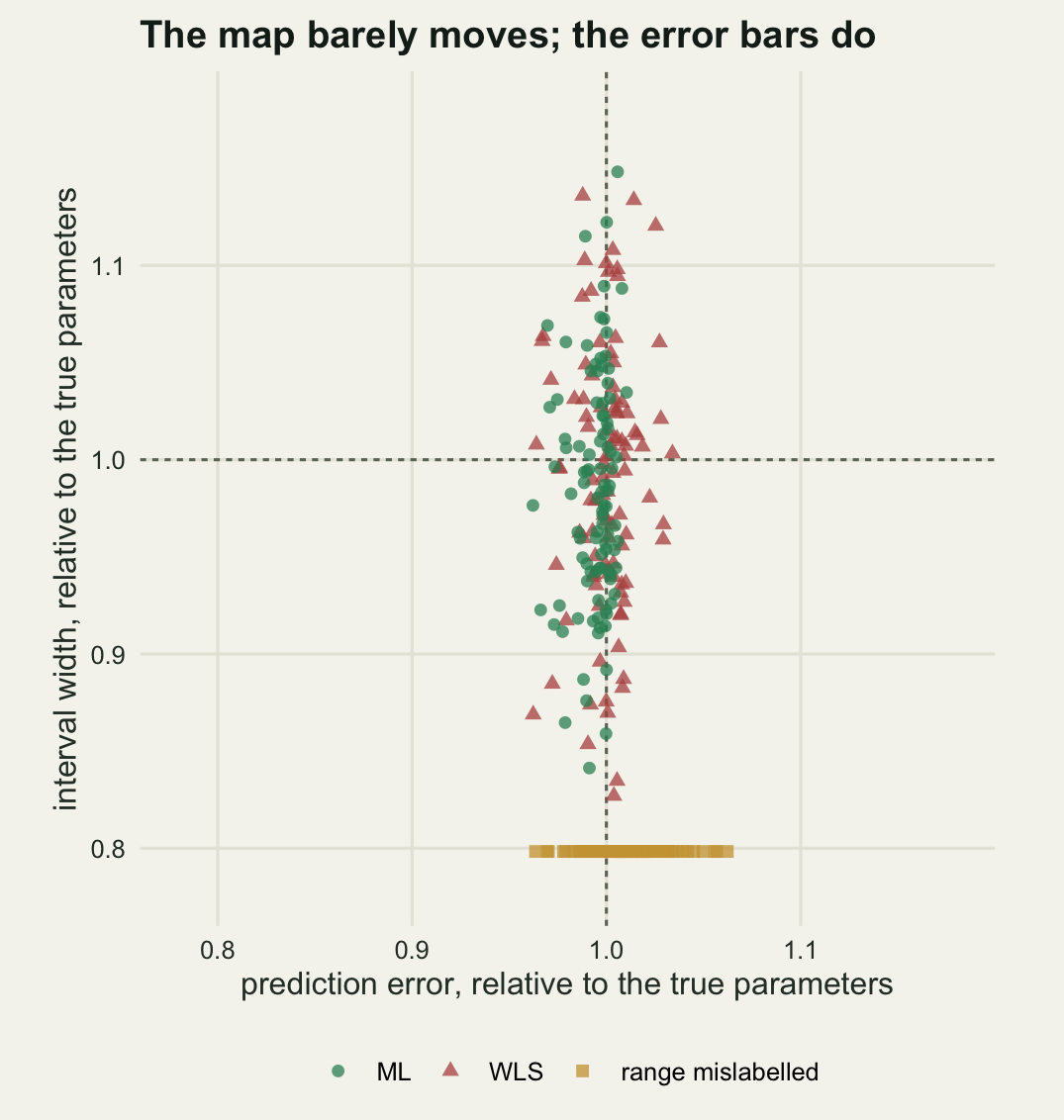
The point prediction is almost indifferent. Cross-validated root mean squared error is 1.56539 with the WLS parameters and 1.5565 with the ML parameters, against 1.5657 with the generating values, a WLS difference of -0.02 per cent. Two estimators whose length-scale estimates differ by a factor of 1.98 in spread produce maps that are the same map. The worst single dataset in the hundred cost WLS 3.4 per cent.
Maximum likelihood came out at -0.588 per cent, which is better than the true parameters. The truth is the best parameter set averaged over realisations of the field, not for the one realisation in front of you, and a fitted length-scale adapts to how wiggly this field happened to come out. The gain is a fraction of a per cent, and it recurs on most of the hundred datasets.
Now the part that was supposed to be the punchline, which came out half right. The expectation going in was that the intervals would be badly served by WLS while the map survived. Average coverage says otherwise: 0.9443 for WLS, 0.9503 for ML and 0.9512 for the truth, against a nominal 0.95. On average the WLS intervals are fine.
What moves is the width, survey by survey. As a standard deviation of the width ratio the vertical spread of the cloud is 0.0675 for WLS and 0.0596 for ML, against a horizontal spread of 0.0139 in the prediction ratio, a factor of 4.9 between the two directions. WLS intervals are typically 6.8 per cent too wide or too narrow on any given survey and average out to the right coverage across surveys. You only run one survey.
The calibration column holds a further reversal. The mean standardised squared residual, which is one if the reported variance is the right variance, is 1 for ML and 0.9832 for the true parameters, and the mean absolute departure from one is 0.0326 against 0.1091. The generating parameters give worse per-survey calibration than the estimates, for the same reason the RMSE went that way.
The fourth arm is unambiguous. Mislabelling the range costs 1.016 per cent in prediction error, which nobody would notice, and takes coverage from 0.9512 to 0.8803. The intervals come out 20.17 per cent too narrow, with a standardised squared residual of 1.5708 instead of one, so the reported variance is short by a factor of about 1.57. A map that looks right, error bars wrong by a fifth, from one conversion error between two names for one number.
What to take away
The variogram and the kernel are the same function, related by \(\gamma(h) = C(0) - C(h)\), and the translation is three lines: nugget to noise variance, partial sill to signal variance, range parameter to length-scale. The correspondence held to 8.88e-16 as an identity, and to 2.15 Monte Carlo standard errors as a statement about the binned estimator over 1500 simulated fields. Simple kriging and the GP posterior mean agreed to 1.07e-14 on 400 grid nodes, and the two prediction variances differed by exactly 0.8, the nugget, because the traditions predict different targets: a new measurement against the underlying function.
The estimator is where they part, and not by a little. Over 200 datasets the binned weighted least squares fit had 1.98 times the standard deviation of maximum likelihood on the length-scale and ran into the bound on 11 datasets against 1. On top of that sampling noise sits a choice with no likelihood counterpart: moving the bin count from 5 to 40 moved the median nugget by a factor of 1.45, and within one dataset the binning alone shifted the nugget by 1.07 of its own value. The likelihood pays for that in cubic arithmetic: 4.17e+10 floating point operations for every evaluation at five thousand plots, and a fit needs of the order of 100 of them.
Two measurements went against the story I set out to write. The map does not care which estimator you used, -0.02 per cent in cross-validated error, and I expected the intervals to care a great deal; average coverage did not, 0.944 for WLS against 0.951 for the true parameters. What degrades is the stability of the interval width from survey to survey, 0.068 as a standard deviation of the ratio. And the true parameters were not the best parameters: the fitted ones beat them on both prediction error and calibration, because a fit adapts to the realisation and the truth cannot. The dictionary error is the one that does damage. A practical range used as a length-scale left prediction essentially unchanged and pulled coverage to 0.88, with intervals 20.2 per cent too narrow.
The honest limit is that the exponential model was correct here, because it generated the fields. Both estimators were fitting the right family, so nothing above speaks to a misspecified one, which is the ordinary situation with real soil or canopy data, and that is where WLS has its one genuine advantage: a binned variogram is a picture, and a curve of the wrong shape through those points is visible, while a likelihood surface offers no comparable view. The second limit is identifiability. Over the 200 datasets the ML partial sill and length-scale were correlated at 0.335, so they move together, though not tightly enough that only their combination is determined. Fixed-domain theory says the ratio \(\sigma_f^2/\ell\) is what the data constrains (Zhang 2004), and its coefficient of variation here was 0.377 against 0.491 for the length-scale alone and 0.251 for the partial sill on its own: better pinned than the length-scale, worse than the partial sill, so the ordering the asymptotic statement implies has not appeared at this sample size. Quote a length-scale from either estimator as a number with a wide interval around it, not as a measured property of the site.
References
Matheron G 1963 Economic Geology 58(8):1246-1266 (10.2113/gsecongeo.58.8.1246)
Cressie N 1985 Journal of the International Association for Mathematical Geology 17(5):563-586 (10.1007/BF01032109)
Mardia KV, Marshall RJ 1984 Biometrika 71(1):135-146 (10.1093/biomet/71.1.135)
Zimmerman DL, Zimmerman MB 1991 Technometrics 33(1):77-91 (10.1080/00401706.1991.10484771)
Lark RM 2000 European Journal of Soil Science 51(4):717-728 (10.1046/j.1365-2389.2000.00345.x)
Zhang H 2004 Journal of the American Statistical Association 99(465):250-261 (10.1198/016214504000000241)
Rasmussen CE, Williams CKI 2006 Gaussian Processes for Machine Learning (ISBN 978-0-262-18253-9)
Diggle PJ, Ribeiro PJ 2007 Model-based Geostatistics (ISBN 978-0-387-32907-9)
Stein ML 1999 Interpolation of Spatial Data: Some Theory for Kriging (ISBN 978-0-387-98629-6)