set.seed(4218)
f_true <- function(x) 1.2*exp(-((x-0.35)^2)/(2*0.09)) - 0.7*exp(-((x-0.78)^2)/(2*0.03)) + 0.25
sig_n_true <- 0.18
gap <- c(0.52, 0.68)                        # an unsampled stretch of the gradient
x  <- sort(runif(58, 0, 1)); x <- x[x < gap[1] | x > gap[2]]
n  <- length(x)
y  <- f_true(x) + rnorm(n, 0, sig_n_true)
ybar <- mean(y); yc <- y - ybar # centre; the GP prior mean is 0 on the residualGaussian process regression from scratch
R
regression
Gaussian processes
ecology tutorial
Fit a Gaussian process in base R along an ecological gradient: the RBF kernel, marginal-likelihood hyperparameters, and a posterior mean with a credible band.
Corrected 30 September 2026: the identifiability section called the weak identification of the length-scale intrinsic and applied an infill result for the Matern family to the squared-exponential kernel; it now says that result does not cover this kernel and that the profile shows a finite-sample weakness.
Suppose you have measured a response along an environmental gradient: an abundance index across a moisture gradient, say, or leaf nitrogen across an elevation transect. The shape is clearly smooth but you have no mechanistic equation for it, the sampling is uneven, and there is a stretch of the gradient nobody visited. You want a flexible fit, and you want the uncertainty to grow honestly where the data thins out.
A Gaussian process (GP) does exactly this. Like the penalised splines behind a generalised additive model, a GP is a flexible smoother, but it is built from a covariance function rather than a basis, and it returns a principled predictive variance at every point. The same machinery, taken onto a map, is the engine behind kriging. Here we fit one from first principles in base R, show that its posterior mean is nothing more exotic than a penalised weighted average, and then look squarely at the part that is easy to gloss over: the length-scale that controls all of this is only weakly pinned down by a single sample.
A distribution over functions
A Gaussian process places a prior directly on the unknown function. The defining property is that the function values at any finite set of locations follow a multivariate normal distribution, with the covariance between two points set by a kernel. We use the squared-exponential (radial basis) kernel,
\[k(x, x') = \sigma_f^2 \, \exp\!\left(-\frac{(x - x')^2}{2\,\ell^2}\right),\]
which says two points are correlated when they are close and independent when they are far apart. The length-scale \(\ell\) controls how quickly that correlation decays (how wiggly the function is allowed to be), and the signal variance \(\sigma_f^2\) sets its vertical scale.
We simulate a smooth but non-trivial response on a standardised gradient, with a deliberate unsampled gap so that the uncertainty has somewhere to grow.
Conditioning on the data
The observations are the function plus independent noise, \(y_i = f(x_i) + \varepsilon_i\) with \(\varepsilon_i \sim \mathcal{N}(0, \sigma_n^2)\). Because everything is jointly normal, the posterior over the function at any set of new locations \(x_\ast\) is again normal, with a closed form. Writing \(K\) for the kernel matrix on the training points and \(K_\ast\) for the cross-covariances to the new points, the posterior mean and variance are
\[\bar f_\ast = K_\ast (K + \sigma_n^2 I)^{-1} y, \qquad \operatorname{Var}(f_\ast) = \sigma_f^2 - K_\ast (K + \sigma_n^2 I)^{-1} K_\ast^{\top}.\]
We never invert the matrix directly. A Cholesky factor gives the same answer with far better numerical behaviour, and it also hands us the log determinant we will need for fitting.
D  <- as.matrix(dist(x))                     # n x n pairwise |x_i - x_j|
kern <- function(D, sf, ell) sf^2 * exp(-(D^2)/(2*ell^2))

nll <- function(par, D, yc) {                # negative log marginal likelihood
  ell <- exp(par[1]); sf <- exp(par[2]); sn <- exp(par[3])
  K   <- kern(D, sf, ell); Ky <- K + diag(sn^2, nrow(K))
  R   <- tryCatch(chol(Ky), error = function(e) NULL)
  if (is.null(R)) return(1e10)
  a   <- backsolve(R, forwardsolve(t(R), yc))
  0.5*sum(yc*a) + sum(log(diag(R))) + 0.5*length(yc)*log(2*pi)
}

predict_gp <- function(xs, x, yc, ybar, sf, ell, sn) {
  K  <- kern(as.matrix(dist(x)), sf, ell) + diag(sn^2, length(x))
  R  <- chol(K); a <- backsolve(R, forwardsolve(t(R), yc))
  Ds <- outer(xs, x, function(u, v) abs(u - v)); Ks <- kern(Ds, sf, ell)
  mu <- as.numeric(Ks %*% a) + ybar
  v  <- forwardsolve(t(R), t(Ks))
  var_f <- sf^2 - colSums(v^2); var_f[var_f < 0] <- 0
  list(mu = mu, sd_f = sqrt(var_f), sd_y = sqrt(var_f + sn^2))
}
Fitting the hyperparameters
The length-scale, signal variance and noise are not set by hand. They are chosen by maximising the marginal likelihood of the data, which after integrating the function out is a plain multivariate normal, \(y \sim \mathcal{N}(0,\, K + \sigma_n^2 I)\). Its log density,
\[\log p(y) = -\tfrac12 y^{\top}(K + \sigma_n^2 I)^{-1} y - \tfrac12 \log\lvert K + \sigma_n^2 I\rvert - \tfrac{n}{2}\log 2\pi,\]
balances fit (the first term) against complexity (the log determinant), so it will not simply chase the noise. We optimise on the log scale to keep every parameter positive.
fit <- optim(c(log(0.15), log(sd(yc)), log(0.2)), nll, D = D, yc = yc,
             method = "BFGS", control = list(maxit = 500))
ell_hat <- exp(fit$par[1]); sf_hat <- exp(fit$par[2]); sn_hat <- exp(fit$par[3])
logML   <- -fit$value
xg  <- seq(-0.15, 1.15, length.out = 300)    # a fine grid, with a little extrapolation
pg  <- predict_gp(xg, x, yc, ybar, sf_hat, ell_hat, sn_hat)
inr <- xg >= min(x) & xg <= max(x)
rmse_gp <- sqrt(mean((pg$mu[inr] - f_true(xg[inr]))^2))
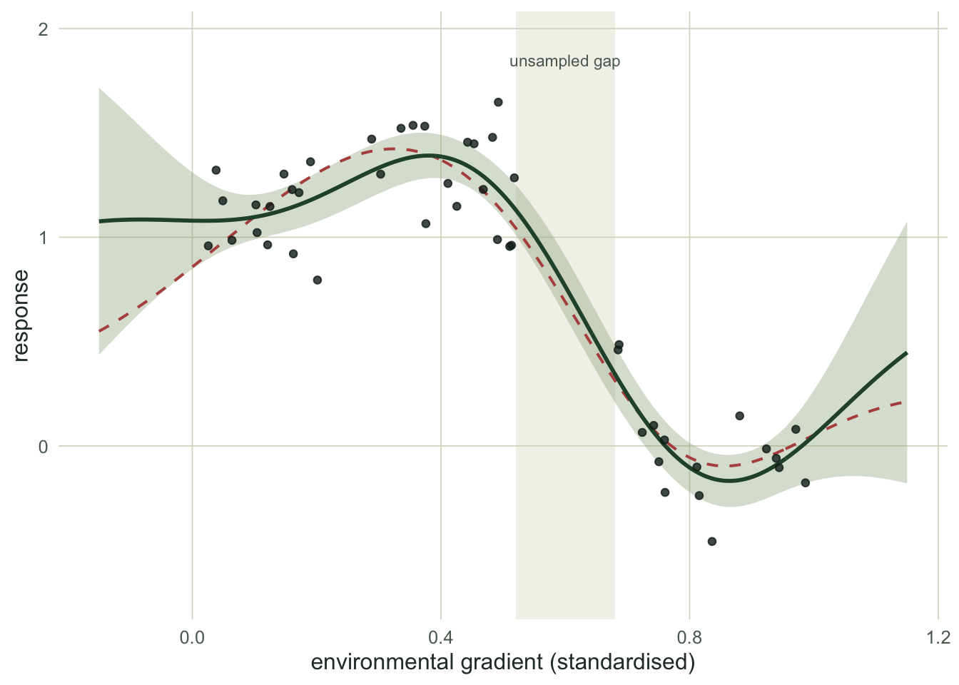
The fit recovers a length-scale of 0.24, a signal SD of 0.59, and a noise SD of 0.19, which is close to the true 0.18. The posterior mean tracks the truth well over the observed span (root mean squared error 0.070), and the band does the useful thing: it stays tight where points are dense and swells across the gap and at the edges, because the kernel has little to lean on there.
What the posterior mean actually is
It is tempting to treat a GP as a black box, but the posterior mean is transparent. Collect the weights \(\alpha = (K + \sigma_n^2 I)^{-1} y\); then \(\bar f_\ast = \sum_i \alpha_i\, k(x_\ast, x_i)\) is a weighted sum of kernels centred on the data. Pull the signal variance out of the kernel and the mean is exactly kernel ridge regression on the correlation kernel \(\tilde K\), penalised by the noise-to-signal ratio \(\lambda = \sigma_n^2 / \sigma_f^2\).
lambda_kr <- sn_hat^2 / sf_hat^2                 # noise-to-signal ratio = ridge penalty
Ktil   <- exp(-(D^2)/(2*ell_hat^2))              # correlation kernel (signal SD set to 1)
a_kr   <- solve(Ktil + diag(lambda_kr, n), yc)
Ds_g   <- outer(xg, x, function(u, v) abs(u - v)); Ktil_s <- exp(-(Ds_g^2)/(2*ell_hat^2))
mu_kr  <- as.numeric(Ktil_s %*% a_kr) + ybar
max_gp_vs_kr <- max(abs(pg$mu - mu_kr))          # agreement to machine precision
The two predictions agree to within floating-point rounding, with penalty \(\lambda =\) 0.10. This is worth holding onto for three reasons. It says a GP is a penalised smoother, the same family as the spline in a GAM, where the length-scale plays the role of the smoothing parameter; the geoadditive view (Kammann and Wand 2003) makes the link precise by writing both as a mixed model. It says the posterior mean is exactly the simple-kriging predictor, the known-mean version of the ordinary kriging used on maps in the kriging tutorial. And it says the length-scale and the signal-to-noise split are the levers that matter, which is where the honesty comes in.
The length-scale is only weakly identified
The marginal likelihood chose a single length-scale, but it did not choose it sharply. If we profile the marginal likelihood over \(\ell\), re-optimising the variances at each value, the curve has a broad rather than a peaked maximum.
ell_grid <- exp(seq(log(0.03), log(0.60), length.out = 60))
prof <- sapply(ell_grid, function(le) {
  o <- optim(c(log(sd(yc)), log(0.2)),
             function(p) nll(c(log(le), p[1], p[2]), D, yc),
             method = "BFGS", control = list(maxit = 300))
  -o$value
})
ell_mle <- ell_grid[which.max(prof)]
within2 <- ell_grid[prof >= max(prof) - 2]       # length-scales within 2 log-ML of the best
ell_lo  <- min(within2); ell_hi <- max(within2); ratio_flat <- ell_hi / ell_lo

refit_at <- function(le) {
  o <- optim(c(log(sd(yc)), log(0.2)),
             function(p) nll(c(log(le), p[1], p[2]), D, yc),
             method = "BFGS", control = list(maxit = 300))
  list(ell = le, sf = exp(o$par[1]), sn = exp(o$par[2]))
}
plo <- refit_at(ell_lo); phi <- refit_at(ell_hi)
glo <- predict_gp(xg, x, yc, ybar, plo$sf, plo$ell, plo$sn)
ghi <- predict_gp(xg, x, yc, ybar, phi$sf, phi$ell, phi$sn)
dense <- inr & (xg < gap[1] | xg > gap[2])
maxdiff_dense <- max(abs(glo$mu[dense] - ghi$mu[dense]))
ig <- which.min(abs(xg - mean(gap)))
diff_gap    <- abs(glo$mu[ig] - ghi$mu[ig])
band_lo_gap <- 2*1.96*glo$sd_f[ig]; band_hi_gap <- 2*1.96*ghi$sd_f[ig]
Every length-scale between 0.14 and 0.34 sits within two log-likelihood units of the best value at 0.24: a factor of 2.4 in the quantity that governs the whole fit. Take the two ends of that plausible range and compare the fits. Their posterior means differ by at most 0.06 where the points are dense, and by 0.10 at the centre of the gap. There the shorter length-scale reports a 95% band 0.47 wide against 0.24 for the longer one.
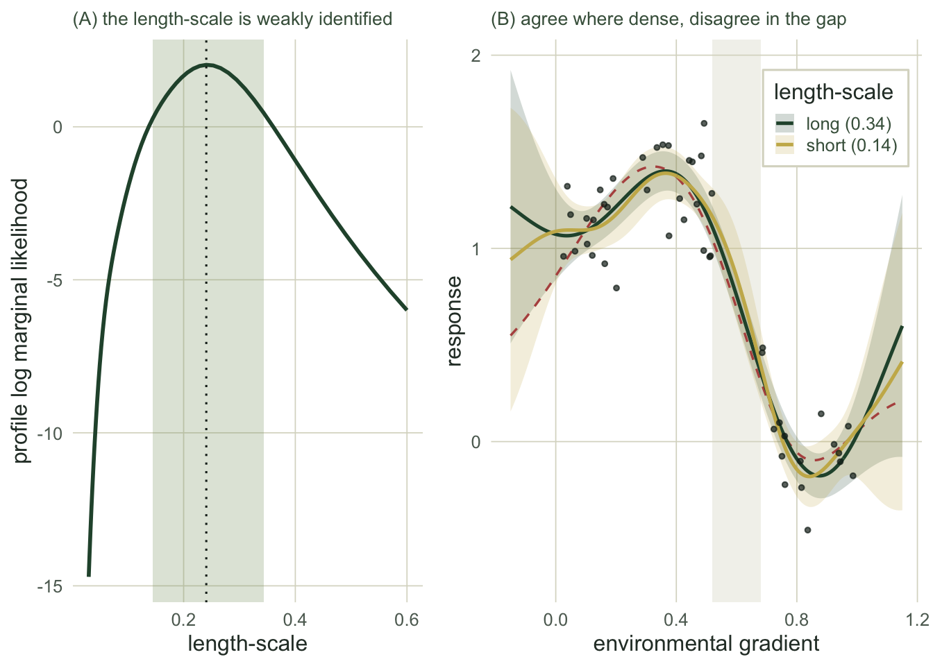
This is not a defect of the code. For the Matern family with a fixed smoothness, Zhang (2004) showed that under denser and denser sampling of a fixed region the variance and the range cannot both be estimated consistently: only a single combination of them, the one that matters for interpolation, is pinned down. The squared-exponential kernel is the limit of that family and is not covered by the proof, so here the result is an analogy; what the profile above shows directly is that this sample pins the length-scale down only loosely. A convergent fit and a tidy point estimate do not imply that the length-scale is identified.
Where this leaves you
A Gaussian process is a genuinely useful flexible smoother: it fits an unknown response without a functional form, and its band grows honestly where the data is sparse, which a bare spline fit does not advertise. But treat the length-scale and the signal-to-noise split as weakly identified quantities rather than settled numbers. The plug-in band conditions on a single hyperparameter estimate, so in data-poor regions it understates the true spread; propagating hyperparameter uncertainty, or at least checking how the fit moves across the plausible range, is the honest habit. And the plug-in variance should not be the only thing you trust: out-of-sample checks, which we take up in checking a predictive model, are what keep it honest. That is the same move that recurs across this site, from the E-value to honest quantile tails: name the modelling choice, and do not read a plug-in interval as the last word.
A Gaussian process is one flexible smoother among several. Local regression reaches a similar fit from a different direction, weighting nearby points rather than placing a prior over functions, and it makes the bias hidden in every smoother easy to see. And when a calibrated interval matters more than a model-based one, conformal prediction wraps any of these fits in a band with a coverage guarantee that does not depend on the length-scale being right. The same idea carried onto a map is kriging: there the distance is measured on the ground, but everything above carries over unchanged.
References
Rasmussen CE, Williams CKI 2006. Gaussian Processes for Machine Learning. MIT Press. ISBN 978-0-262-18253-9.
Zhang H 2004. Journal of the American Statistical Association 99(465):250-261 (10.1198/016214504000000241).
Kammann EE, Wand MP 2003. Journal of the Royal Statistical Society Series C 52(1):1-18 (10.1111/1467-9876.00385).
Dormann CF, McPherson JM, Araujo MB, and others 2007. Ecography 30(5):609-628 (10.1111/j.2007.0906-7590.05171.x).