set.seed(4219)
f_true <- function(x) 0.50*x +
  0.90*exp(-((x-0.30)^2)/(2*0.008)) +               # sharp bump (sd ~ 0.09)
  0.50*exp(-((x-0.70)^2)/(2*0.040))                 # broad bump (sd ~ 0.20)
sig_true <- 0.12
n  <- 120
x  <- sort(runif(n))
y  <- f_true(x) + rnorm(n, 0, sig_true)
xg <- seq(0, 1, length.out = 400)

gk <- function(u) exp(-0.5*u^2)                        # Gaussian kernel
nw <- function(x0, x, y, h){ w <- gk((x - x0)/h); sum(w*y)/sum(w) } # local constantLocal regression from scratch
R
regression
nonparametric
ecology tutorial
Nadaraya-Watson and local linear regression in base R, bandwidth chosen by cross-validation, and why a variance-only band under-covers where the curve bends.
Corrected 15 October 2026: the bandwidth paragraph called the values it quotes the fitted peak height; they are the fitted values at the true peak, and the text now says so. The closing section said the variance-only band is centred low wherever the response curves sharply; it is centred low at a peak but high in a valley, where the smoothing bias has the opposite sign, and it now says so.
Corrected 7 October 2026: the introduction and the coverage figure’s caption said that the band’s real coverage falls well short wherever the curve bends; it does so around the sharp bump, where the curve bends most, and hardly moves at the broad one, and the text now says so. The alt text of the bandwidth panel described a U-shaped curve with a wide trough; it now describes the curve as drawn, lowest near the left end of the axis.
Corrected 30 September 2026: the closing section said conformal prediction supplies the calibrated band this post needs; it now says conformal intervals cover a new observation rather than the mean curve, and that their coverage is averaged over the gradient, so they do not by themselves fix the under-coverage at the peak. The coverage calculation also treated this sample’s noise estimate as the true noise level; it now uses the true noise level of the simulation, which raises the computed coverage somewhat without changing the conclusion.
Corrected 27 September 2026: panel B of the coverage figure plotted single fits to the noisy data, in which the local constant fit happened to sit closer to the truth than the local linear one, the opposite of what its caption said; it now plots the expected fits (each smoother applied to the true mean), which show the edge bias the text describes.
Updated 27 September 2026: a new section, The smoother you did not choose, measures what geom_smooth() fits by default on this curve: below 1000 rows a loess with a fixed span that misses the sharp peak by more than a quarter of its height, which is the smoother applied to the truth rather than noise, and from 1000 rows a gam that still falls short on a narrower peak.
A Gaussian process fits a curve by putting a prior over functions. Local regression reaches a similar place from the opposite direction: to estimate the response at a point, just fit a simple model to the nearby data, weighting points by how close they are. No global functional form, no basis, only a kernel and a bandwidth. It is the idea behind LOESS, and it is worth building by hand because the machinery makes one honest lesson unavoidable: the usual pointwise confidence band is built from variance alone, and where the curve bends sharply it is centred on a biased estimate, so its real coverage is well short of what the label claims.
Local averaging
The simplest local estimator is a weighted average. To predict the response at a target \(x_0\), weight each observation by a kernel of its distance and take the weighted mean. This is the Nadaraya-Watson estimator, a local constant fit:
\[\hat m(x_0) = \frac{\sum_i K\!\big(\tfrac{x_i - x_0}{h}\big)\, y_i}{\sum_i K\!\big(\tfrac{x_i - x_0}{h}\big)}.\]
The bandwidth \(h\) is the one knob that matters: small \(h\) tracks the data closely but is noisy, large \(h\) is smooth but blurs real structure. We use a Gaussian kernel.
From local constant to local linear
The weighted average has a weakness at the edges. Near a boundary the kernel is one-sided, so if the curve has a slope there, the average is pulled towards the interior and the fit is biased. The fix is to fit a local straight line instead of a local level: run a weighted least squares of \(y\) on \(x - x_0\) and read off the intercept. Writing the design as \(X = [1, x - x_0]\) and the kernel weights as a diagonal \(W\), the estimate is a linear combination of the responses, \(\hat m(x_0) = e_1^\top (X^\top W X)^{-1} X^\top W\, y\), so we can extract the effective weight each observation carries. Collecting those weight vectors for every fitted point gives the smoother matrix \(L\) with \(\hat y = L y\), which we will need for both cross-validation and the confidence band.
ll_wts <- function(x0, x, h){                          # local linear effective weights
  w <- gk((x - x0)/h); X <- cbind(1, x - x0)
  XtW <- t(X * w); A <- XtW %*% X
  as.numeric((solve(A) %*% XtW)[1, ])
}
ll_fit <- function(xt, x, y, h){
  L <- t(vapply(xt, ll_wts, numeric(length(x)), x = x, h = h))
  list(mu = as.numeric(L %*% y), L = L)
}
Choosing the bandwidth
The smoother matrix gives leave-one-out cross-validation almost for free: the deleted residual at point \(i\) is the ordinary residual divided by \(1 - L_{ii}\), so we never refit. We minimise the cross-validation score over a grid of bandwidths.
cv_h <- function(h){
  L <- t(vapply(x, ll_wts, numeric(n), x = x, h = h))
  fit <- as.numeric(L %*% y); dL <- diag(L)
  mean(((y - fit)/(1 - dL))^2)
}
h_grid <- exp(seq(log(0.015), log(0.20), length.out = 40))
cv <- sapply(h_grid, cv_h)
h_cv <- h_grid[which.min(cv)]
cv_thr <- min(cv)*1.05; h_band <- h_grid[cv <= cv_thr]     # within 5% of the best score
h_lo <- min(h_band); h_hi <- max(h_band); h_ratio <- h_hi/h_lo
Cross-validation picks a bandwidth of 0.029, giving a fit with about 15 effective degrees of freedom. We fit at that bandwidth and attach the textbook variance-only band, using the residual variance and the row norms of the smoother matrix.
onx <- ll_fit(x, x, y, h_cv); L <- onx$L
nu  <- sum(diag(L))
sig2 <- sum((y - onx$mu)^2)/(n - nu)
fg  <- ll_fit(xg, x, y, h_cv); Lg <- fg$L
sd_g <- sqrt(sig2 * rowSums(Lg^2))                     # variance only, ignores bias
hw_g <- 1.96*sd_g; lo_g <- fg$mu - hw_g; hi_g <- fg$mu + hw_g
tru_g <- f_true(xg); ftx <- f_true(x)
inr <- xg >= min(x) & xg <= max(x)
Setup: packages, colours and plot theme
suppressPackageStartupMessages(library(ggplot2))
theme_te <- function() theme_minimal(base_size = 12) +
  theme(panel.grid.minor = element_blank(),
        panel.grid.major = element_line(colour = "#dad9ca", linewidth = 0.3),
        axis.title = element_text(colour = "#2c3a31"), axis.text = element_text(colour = "#5d6b61"),
        plot.subtitle = element_text(colour = "#46604a", size = 10),
        plot.background = element_rect(fill = "#f5f4ee", colour = NA),
        panel.background = element_rect(fill = "#f5f4ee", colour = NA))
forest <- "#275139"; terra <- "#b5534e"
dg <- data.frame(x = xg, mu = fg$mu, lo = lo_g, hi = hi_g, tru = tru_g)
pA <- ggplot() +
  geom_point(data = data.frame(x, y), aes(x, y), colour = "#93a87f", alpha = 0.55, size = 1.4) +
  geom_ribbon(data = dg, aes(x, ymin = lo, ymax = hi), fill = "#93a87f", alpha = 0.30) +
  geom_line(data = dg, aes(x, tru), colour = "#16241d", linetype = "dashed", linewidth = 0.8) +
  geom_line(data = dg, aes(x, mu), colour = forest, linewidth = 1.1) +
  labs(x = "environmental gradient", y = "response", subtitle = "(A) local linear fit and 95% band") +
  theme_te()
dcv <- data.frame(h = h_grid, cv = cv)
pB <- ggplot(dcv, aes(h, cv)) +
  annotate("rect", xmin = h_lo, xmax = h_hi, ymin = -Inf, ymax = Inf, fill = "#93a87f", alpha = 0.30) +
  geom_line(colour = forest, linewidth = 1) +
  geom_vline(xintercept = h_cv, colour = "#5d6b61", linetype = "dotted") +
  labs(x = "bandwidth", y = "leave-one-out CV score", subtitle = "(B) the bandwidth is weakly pinned") +
  theme_te()
grid::pushViewport(grid::viewport(layout = grid::grid.layout(1, 2)))
print(pA, vp = grid::viewport(layout.pos.row = 1, layout.pos.col = 1))
print(pB, vp = grid::viewport(layout.pos.row = 1, layout.pos.col = 2))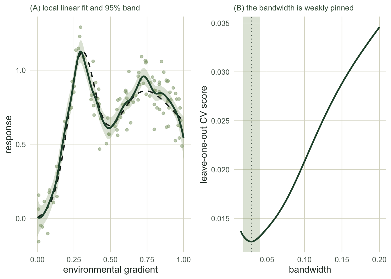
Why the band under-covers
The band above is honest about noise and silent about bias. To see the bias without any noise getting in the way, apply the smoother to the true mean function: the result is the fit you would get on average, and it differs from the truth by exactly the smoothing bias.
efit_g <- as.numeric(Lg %*% ftx)                       # expected fit = smoother on the truth
bias_g <- efit_g - tru_g                               # exact smoothing bias
ipk <- which.max(tru_g); xpk <- xg[ipk]                # the sharp optimum
sd_true_g <- sig_true * sqrt(rowSums(Lg^2))            # sampling sd of the fit (true noise sd)
bias_pk <- bias_g[ipk]; se_pk <- sd_true_g[ipk]; bias_in_se_pk <- abs(bias_pk)/se_pk
## true coverage of the NOMINAL 95% band over repeated samples: the fit is centred at truth + bias
cover_g  <- pnorm(1.96 - bias_g/sd_true_g) - pnorm(-1.96 - bias_g/sd_true_g)
cover_pk <- cover_g[ipk]; min_cov <- min(cover_g[inr])
frac_undercover <- mean(cover_g[inr] < 0.90)
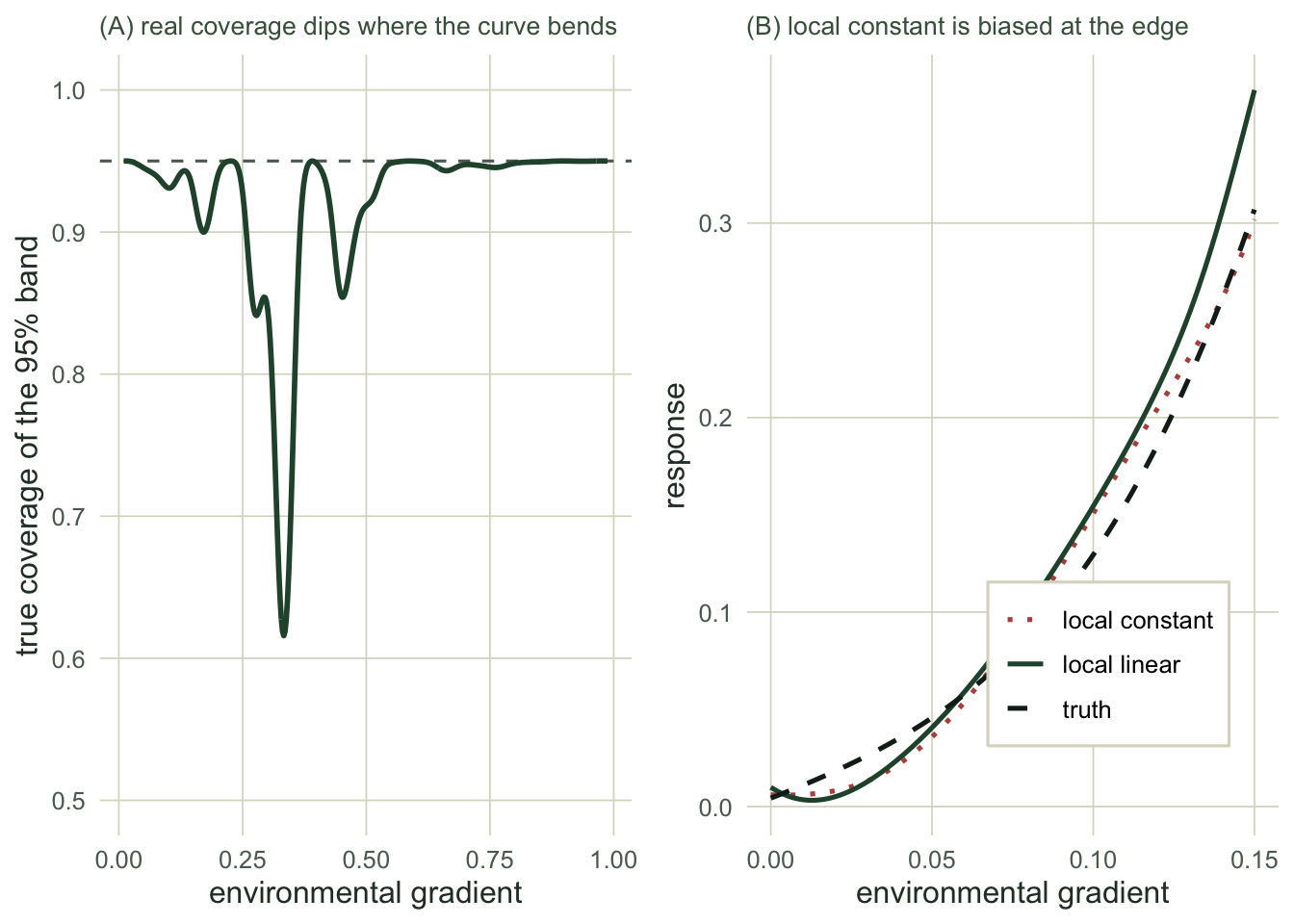
At the sharp peak the fit sits 0.046 below the truth, which is 1.0 standard errors. The band is not too narrow; it is centred in the wrong place. A pointwise interval labelled 95 per cent therefore contains the true value at the peak only about 83 per cent of the time over repeated samples, and just past the crest its true coverage falls to 69 per cent. Across the interior, 14 per cent of the grid has real coverage below 90 per cent. More data at this same cross-validated bandwidth would not fix it, because the missing piece is bias, not variance.
The bandwidth itself is barely pinned down. Bandwidths from 0.018 to 0.041, a 2.2-fold range, all fit within five per cent of the best cross-validation score, and across that range the fitted value at the true peak swings from 1.04 to 1.13. How smooth the curve should be is a judgement the data leaves largely open.
Finally, the boundary is where the local constant estimator earns its bad name.
xb <- xg[xg <= 0.08]                                   # left edge, where the curve has a slope
nw_eb <- sapply(xb, function(x0){ w <- gk((x - x0)/h_cv); sum(w*ftx)/sum(w) })   # NW on the truth
Lb <- t(vapply(xb, ll_wts, numeric(n), x = x, h = h_cv)); ll_eb <- as.numeric(Lb %*% ftx)
bias_nw_0 <- abs(nw_eb[1] - f_true(xb[1])); bias_ll_0 <- abs(ll_eb[1] - f_true(xb[1]))
Right at the left edge, where the response is rising, the local constant fit is off by 0.013 while the local linear fit is off by only 0.003. A one-sided average cannot follow a trend; a local line can, which is why local linear is the sensible default.
The smoother you did not choose: geom_smooth()
In R the quickest local regression is the line geom_smooth() draws when it is given no method. The same idea as above tells you what that line fits on this curve: read the plotted curve back out with layer_data(), match it to a plain loess() call, then apply that smoother to the true mean function.
sm_msg <- character()
keep_msg <- function(expr) withCallingHandlers(expr, message = function(m) {
  sm_msg <<- c(sm_msg, conditionMessage(m)); invokeRestart("muffleMessage") })
ld_def <- keep_msg(layer_data(ggplot(data.frame(x, y), aes(x, y)) + geom_smooth(), 1))
cat(sm_msg, sep = "\n")                                # the message ggplot2 prints
`geom_smooth()` using method = 'loess' and formula = 'y ~ x'lo_def <- loess(y ~ x, span = 0.75) # loess default degree: 2 (local quadratic)
stopifnot(formals(loess)$degree == 2, isTRUE(all.equal(ld_def$y, # the plotted curve is this loess
as.numeric(predict(lo_def, data.frame(x = ld_def$x))), tolerance = 1e-6)))
fit_def_pk <- predict(lo_def, data.frame(x = xpk)) # the default on these data, at the peak
ef_def_pk <- predict(loess(ftx ~ x, span = 0.75), data.frame(x = xpk)) # smoother on the truth
bias_def_pk <- ef_def_pk - tru_g[ipk]
xe_n <- seq(0, 1, length.out = n); ef_def_even <- predict(loess(f_true(xe_n) ~ xe_n, span = 0.75), data.frame(xe_n = xpk))
set.seed(2191) # own seed, so no later draw moves; 300 fresh noise draws at the same x
mc_def <- replicate(300, predict(loess(I(ftx + rnorm(n, 0, sig_true)) ~ x, span = 0.75), data.frame(x = xpk)))On 120 rows the default is a loess with span 0.75 (every local fit uses three quarters of the data) and a local quadratic; the guard checks this against the curve ggplot2 actually draws (ggplot2 4.0.3 here; the check rests on the drawn curve, not on the wording of the message). At the sharp peak the default curve sits at 0.793 against a true 1.124. This is not bad luck in the noise. A loess with the default gaussian family is linear in \(y\), like the smoother matrix above, so its average fit is the smoother applied to the truth: 0.813, a shortfall of 35 per cent of the bump’s 0.9 height. Averaging the default over 300 fresh noise draws at the same \(x\) gives 0.812 (Monte Carlo SE 0.001), which reproduces it. The cross-validated local linear fit of this post has an expected peak of 1.078; the default’s bias is 6.8 times as large. Part of the shortfall is where these 120 x values happen to fall: on an evenly spaced design of the same size the same arithmetic gives 0.876, 28 per cent of the bump short, and because the span is a fraction of the rows, that figure hardly changes with the number of rows (compare the 999-row value below).
The rule changes with the size of the largest group. From 1000 rows ggplot2 fits mgcv::gam(y ~ s(x, bs = "cs"), method = "REML") instead, a penalised spline whose wiggliness is estimated from the data (see GAM species response curves).
f_narrow <- function(x) 0.50*x + 0.90*exp(-((x-0.30)^2)/(2*0.0016)) +  # sharp bump sd 0.04
  0.50*exp(-((x-0.70)^2)/(2*0.040))
xpn <- xg[which.max(f_narrow(xg))]
draw_fit <- function(f, m, x0, guard = FALSE) {        # the default's value at x0 on m rows
  dd <- data.frame(x = sort(runif(m))); dd$y <- f(dd$x) + rnorm(m, 0, sig_true)
  sm <- if (m < 1000) loess(y ~ x, data = dd, span = 0.75) else
    mgcv::gam(y ~ s(x, bs = "cs"), method = "REML", data = dd)
  if (guard) { ld <- keep_msg(layer_data(ggplot(dd, aes(x, y)) + geom_smooth(), 1))
    stopifnot(isTRUE(all.equal(ld$y, as.numeric(predict(sm, data.frame(x = ld$x))),
                               tolerance = 1e-6))) }
  as.numeric(predict(sm, data.frame(x = x0)))
}
set.seed(2192)
invisible(draw_fit(f_true, 999, xpk, TRUE)); invisible(draw_fit(f_true, 1000, xpk, TRUE))
cat(tail(sm_msg, 1), sep = "\n")
`geom_smooth()` using method = 'gam' and formula = 'y ~ s(x, bs = "cs")'sw <- sapply(c(999, 1000), function(m) cbind(host = replicate(50, draw_fit(f_true, m, xpk)),
narrow = replicate(50, draw_fit(f_narrow, m, xpn))),
simplify = "array") # 50 draws x bump x rows
sw_mean <- apply(sw, 2:3, mean); sw_se <- apply(sw, 2:3, sd)/sqrt(dim(sw)[1])
xe <- seq(0, 1, length.out = 999) # smoother on the truth, even 999-row design
ef_999 <- c(predict(loess(f_true(xe) ~ xe, span = 0.75), data.frame(xe = xpk)),
predict(loess(f_narrow(xe) ~ xe, span = 0.75), data.frame(xe = xpn)))On 999 rows the default still averages 0.876 at this post’s peak; on 1000 rows, same code, it averages 1.108 against the true 1.124 (50 draws each, Monte Carlo SE at most 0.009). The gam does not recover a peak in general, though. Narrow the bump to a standard deviation of 0.04 and its true height is 1.119: 999 rows give 0.563 and 1000 rows 0.861, still 29 per cent of the bump short. The 999-row averages are the smoother-on-truth arithmetic again: loess on the noise-free curves over an evenly spaced 999-row design gives 0.874 and 0.562 (the draws use random x, so the match is close rather than exact). The gam chooses its own smoothness from each noisy sample, so it is not linear in \(y\) and its numbers are simulation averages only.
The repair is the one this post already used: state the method and choose the smoothing by cross-validation rather than inherit it.
spans <- seq(0.15, 0.75, by = 0.05); inner <- 2:(n - 1)   # loess will not extrapolate to the ends
cv_span <- sapply(spans, function(s) mean(sapply(inner, function(i)
  (y[i] - predict(loess(y ~ x, span = s, subset = -i), data.frame(x = x[i])))^2)))
span_cv <- spans[which.min(cv_span)]
ld_cv <- layer_data(ggplot(data.frame(x, y), aes(x, y)) +
                      geom_smooth(method = "loess", span = span_cv, formula = y ~ x), 1)
stopifnot(isTRUE(all.equal(ld_cv$y, as.numeric(predict(loess(y ~ x, span = span_cv),
                                                        data.frame(x = ld_cv$x))), tolerance = 1e-6)))
ef_cv_pk <- predict(loess(ftx ~ x, span = span_cv), data.frame(x = xpk))
Leave-one-out cross-validation over the span picks 0.20, and geom_smooth(method = "loess", span = span_cv, formula = y ~ x) with that value has an expected peak of 1.107. That span is a property of these data and this curve, not a value to copy, and it is weakly pinned, as the bandwidth was: the next span up, 0.25, scores only 1.1 per cent worse in cross-validation.
Where this leaves you
Local regression is an easy, transparent smoother, and local linear is the version to reach for because it behaves at the edges. But read its pointwise band with the same caution as any plug-in interval. It accounts for variance and ignores the smoothing bias, so where the response curves sharply the interval is centred off the curve, low at a peak and high in a valley, and its true coverage falls well below the label, here to around 69 per cent. Undersmoothing on purpose shrinks the bias but widens the band and defeats the point; the honest response is to stop trusting a variance-only interval as if it were calibrated.
Conformal prediction offers a different kind of guarantee: a prediction interval for a new observation around any of these fits, this one or the Gaussian process, whose coverage holds in finite samples without getting the smoothness or the bias right. That coverage is an average over the whole gradient rather than a promise at each point, so it does not by itself repair the shortfall at the peak, and it covers a new observation, not the mean curve. And whichever interval you use, the honest final step is to check its coverage on held-out data rather than trust the formula.
References
Cleveland WS 1979. Journal of the American Statistical Association 74(368):829-836 (10.1080/01621459.1979.10481038).
Cleveland WS, Devlin SJ 1988. Journal of the American Statistical Association 83(403):596-610 (10.1080/01621459.1988.10478639).
Fan J, Gijbels I 1996. Local Polynomial Modelling and Its Applications. Chapman and Hall/CRC. ISBN 978-0-412-98321-4.
Wasserman L 2006. All of Nonparametric Statistics. Springer, New York. ISBN 978-0-387-25145-5.