set.seed(4220)
f_true <- function(x) 0.40 + 1.2*x - 1.0*x^2 + 0.45*sin(6*x)   # smooth mean
sig    <- function(x) 0.05 + 0.40*x                            # noise grows across the gradient
gen    <- function(n){ x <- runif(n); data.frame(x = x, y = f_true(x) + rnorm(n, 0, sig(x))) }

base_fit  <- function(tr, deg = 6) lm(y ~ poly(x, deg), data = tr)
base_pred <- function(m, xnew) as.numeric(predict(m, newdata = data.frame(x = xnew)))
alpha <- 0.10

split_conf <- function(tr, ca, xnew, alpha = 0.10){
  m <- base_fit(tr); r <- abs(ca$y - base_pred(m, ca$x))
  k <- ceiling((1 - alpha)*(nrow(ca) + 1)); q <- sort(r)[min(k, length(r))]
  mu <- base_pred(m, xnew); list(mu = mu, lo = mu - q, hi = mu + q, q = q)
}Conformal prediction intervals from scratch
R
prediction
uncertainty
ecology tutorial
Split and locally adaptive conformal intervals in base R: a distribution-free coverage guarantee, and the honest gap between marginal and conditional coverage.
Corrected 7 October 2026: the introduction called conformal prediction the constructive answer to the under-covering bands of the two previous posts and said it covers the truth; it covers a new observation, not the mean curve the local regression band was for, as that post now says, and the introduction now says so.
Corrected 30 September 2026: the post put the coverage a shade above nominal down to the conservatism of the finite-sample guarantee; at this calibration size that conservatism is far smaller than the excess, so the text now attributes most of it to Monte Carlo noise.
The two previous tutorials ended on the same worry. A Gaussian process hands you a plug-in band that leans on a length-scale it cannot quite pin down, and a local regression hands you a variance-only band that is centred on a biased fit. Both under-cover, and both do so in a way that depends on the model being roughly right. Conformal prediction offers a different kind of guarantee: a band around any model’s predictions that is guaranteed to cover a new observation at the nominal rate in finite samples, with no assumption on the shape of the regression function or the distribution of the noise. It covers observations, not the mean curve that the local regression band was for. The only price is one honest caveat, which this post makes concrete: the guarantee is about coverage on average, not coverage everywhere.
Split conformal
The idea is disarmingly simple. Split the data into a training part and a calibration part. Fit any model you like on the training part. On the calibration part, record how wrong the model is at each point, the absolute residual, and call these the conformity scores. To predict at a new point, take the model’s prediction and pad it by the appropriate quantile of those calibration scores. Because the calibration and test points are exchangeable, a new residual is equally likely to land at any rank among the calibration residuals, and that fact alone pins the coverage: with the quantile taken at level \(\lceil (1-\alpha)(n_{\text{cal}}+1)\rceil / n_{\text{cal}}\), the interval covers the truth with probability at least \(1-\alpha\), whatever the model and whatever the data.
We simulate a response whose noise grows across the gradient, and deliberately use a plain polynomial as the base learner so that any coverage we see comes from conformal, not from a well-chosen model.
The guarantee holds
To see that the coverage is real and not an artefact of one lucky split, we repeat the whole procedure many times, each on fresh data, and record whether a fresh test point falls in the interval.
R <- 3000; hit <- numeric(R)
for (b in 1:R){
  d <- gen(200); tr <- d[1:100, ]; ca <- d[101:200, ]
  xt <- runif(1); yt <- f_true(xt) + rnorm(1, 0, sig(xt))
  sc <- split_conf(tr, ca, xt, alpha); hit[b] <- (yt >= sc$lo) && (yt <= sc$hi)
}
marg_cov <- mean(hit)
Across 3000 repetitions the interval covered the truth 90.7 per cent of the time, right at the nominal 90 per cent (a shade above; the finite-sample guarantee is conservative by much less than that at this calibration size, so most of the excess is Monte Carlo noise). No distributional assumption was used, and the base model is a crude polynomial. That is the appeal of conformal inference: valid coverage for free, wrapped around whatever you already fit.
Marginal is not conditional
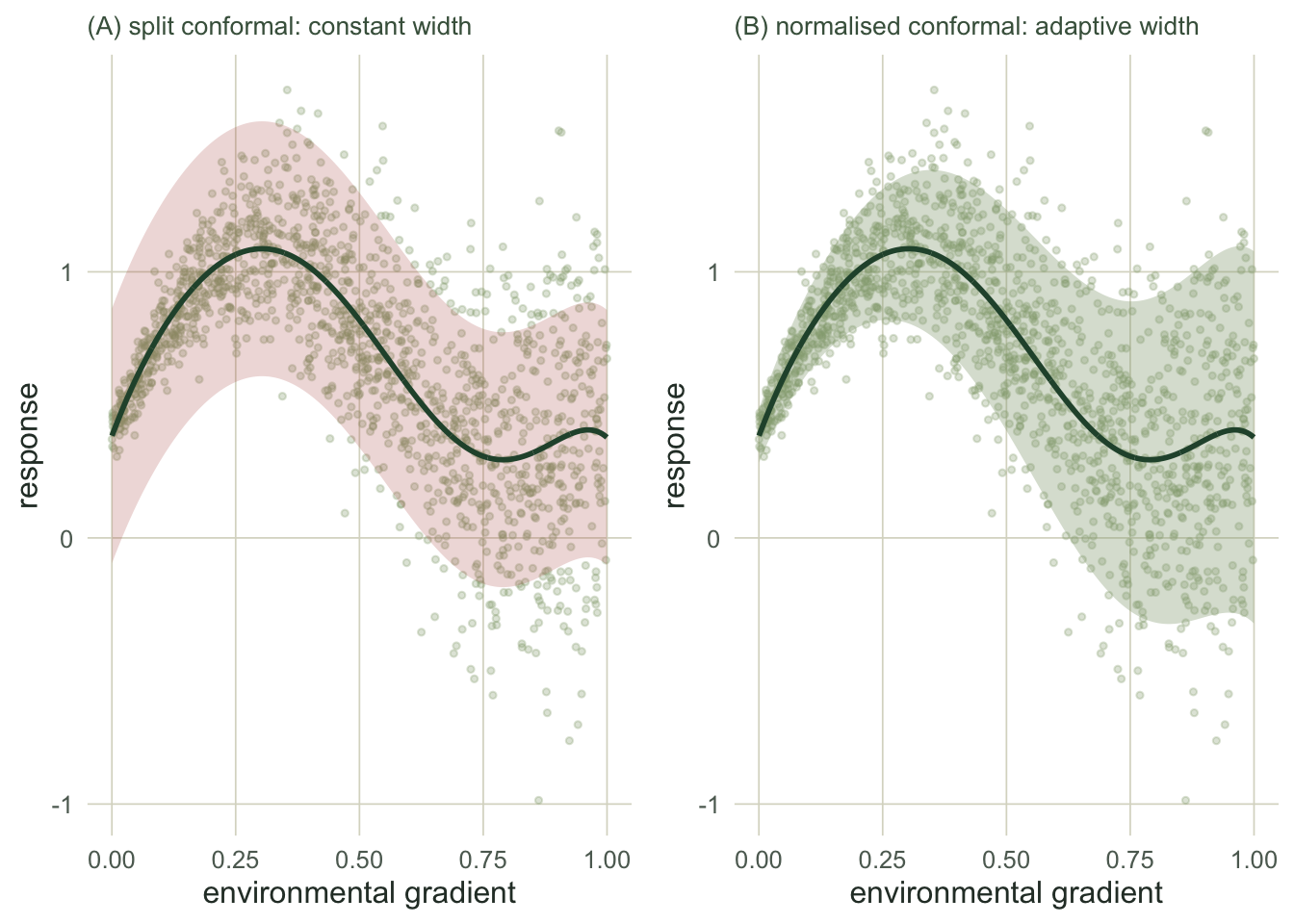
Here is the caveat. Split conformal pads every prediction by the same quantile, so the band has constant width. When the noise varies across the gradient, a single width cannot be right everywhere: it is too wide where the data is quiet and too narrow where the data is loud. The average coverage is still correct, but it is bought by over-covering the easy region and under-covering the hard one.
A cheap remedy is to let the width breathe. Normalised conformal scales each residual by an estimate of the local spread before taking the quantile, so the band widens where the model is typically more wrong. It keeps the marginal guarantee and greatly improves the balance across regions.
norm_conf <- function(tr, ca, xnew, alpha = 0.10){
  m <- base_fit(tr); rtr <- abs(tr$y - base_pred(m, tr$x))
  smod <- lm(log(rtr + 1e-3) ~ poly(x, 4), data = data.frame(x = tr$x, rtr = rtr))
  s <- function(xx) exp(as.numeric(predict(smod, newdata = data.frame(x = xx)))) + 1e-3
  r <- abs(ca$y - base_pred(m, ca$x)) / s(ca$x)
  k <- ceiling((1 - alpha)*(nrow(ca) + 1)); q <- sort(r)[min(k, length(r))]
  mu <- base_pred(m, xnew); sw <- s(xnew); list(mu = mu, lo = mu - q*sw, hi = mu + q*sw)
}

D <- gen(4500); tr <- D[1:1500, ]; ca <- D[1501:3000, ]; te <- D[3001:4500, ]
sc <- split_conf(tr, ca, te$x, alpha); nc <- norm_conf(tr, ca, te$x, alpha)
cov_s <- (te$y >= sc$lo) & (te$y <= sc$hi); cov_n <- (te$y >= nc$lo) & (te$y <= nc$hi)
bins <- cut(te$x, seq(0, 1, 0.2), include.lowest = TRUE)
covbin_s <- tapply(cov_s, bins, mean); covbin_n <- tapply(cov_n, bins, mean)
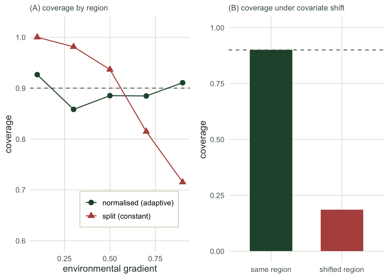
The split band covers 89 per cent overall but its coverage runs from 72 per cent in the noisy right-hand fifth up to 100 per cent in the quiet left-hand fifth. The normalised band covers 89 per cent overall and holds between 86 and 93 per cent across the same bins: its width grows from about 0.31 on the left to about 1.32 on the right, tracking the spread the constant band ignored.
When exchangeability fails
The guarantee rests on one assumption: the calibration and test points are exchangeable, drawn from the same distribution. Break that and the coverage goes with it. Suppose we calibrate only on the low end of the gradient and then predict on the high end, where both the mean and the noise are different, a covariate shift of the kind that spatial and temporal data serve up constantly.
Dl <- D[D$x <= 0.7, ]; Dr <- D[D$x > 0.7, ]              # calibrate low-x, predict high-x
h  <- floor(nrow(Dl)/2); trL <- Dl[1:h, ]; caL <- Dl[(h+1):nrow(Dl), ]
scL <- split_conf(trL, caL, Dr$x, alpha)
cov_shift <- mean(Dr$y >= scL$lo & Dr$y <= scL$hi)
idx <- sample(nrow(Dl)); t3 <- floor(nrow(Dl)/3)          # in-distribution comparison
trI <- Dl[idx[1:t3], ]; caI <- Dl[idx[(t3+1):(2*t3)], ]; teI <- Dl[idx[(2*t3+1):nrow(Dl)], ]
scI <- split_conf(trI, caI, teI$x, alpha); cov_indist <- mean(teI$y >= scI$lo & teI$y <= scI$hi)
Calibrated and tested on the same region, coverage sits at the expected 90 per cent. Calibrated on the low end and pushed to the high end, it collapses to 19 per cent: the residual quantile learned from a quiet region is far too small for a loud one. Conformal does not detect the shift; it simply assumes it away, and the coverage guarantee is void the moment the assumption is.
Where this leaves you
Conformal prediction is the honest default for an interval you actually want to trust. It wraps any model, the Gaussian process, the local regression, a random forest, and turns it into a band with a finite-sample coverage guarantee that does not depend on the model being correct. When you need a prediction interval and cannot vouch for the noise model, reach for it.
Two things to keep in view. First, the guarantee is marginal, not conditional: a constant-width band can hide large swings in coverage across the data, so use normalised conformal, or its relatives like conformalised quantile regression and group-wise (Mondrian) conformal, when different regions deserve different widths. Second, it all rests on exchangeability. Ecological data rarely obliges: spatial autocorrelation, temporal trends and sampling that shifts across a gradient all break it, and there are conformal variants built for dependent and shifted data when they do. Either way, the closing move is the same one this series keeps returning to: do not take a coverage number on faith, check it on held-out data.
References
Vovk V, Gammerman A, Shafer G 2005. Algorithmic Learning in a Random World. Springer, New York. ISBN 978-0-387-00152-4.
Lei J, G’Sell M, Rinaldo A, Tibshirani RJ, Wasserman L 2018. Journal of the American Statistical Association 113(523):1094-1111 (10.1080/01621459.2017.1307116).
Barber RF, Candes EJ, Ramdas A, Tibshirani RJ 2021. The Annals of Statistics 49(1):486-507 (10.1214/20-AOS1965).
Angelopoulos AN, Bates S 2023. Foundations and Trends in Machine Learning 16(4):494-591 (10.1561/2200000101).