Checking a quantile regression

Crossing lines, mechanical in-sample calibration, and a tail slope that rests on three points. The diagnostics that keep a quantile fit honest.

A quantile fit can look convincing and still mislead. Independent fits at different levels can cross, which is impossible for real quantiles. The in-sample calibration that seems to validate a fit is guaranteed by the fitting itself and proves nothing about a new sample. And the upper-tail slope that carries the ecological story is estimated from the thin edge of the data, so its uncertainty grows fast as you push toward the extremes. This post, the last in the cluster, works through the three diagnostics that matter and states the honest limit they share with the rest of this blog.

Crossing lines

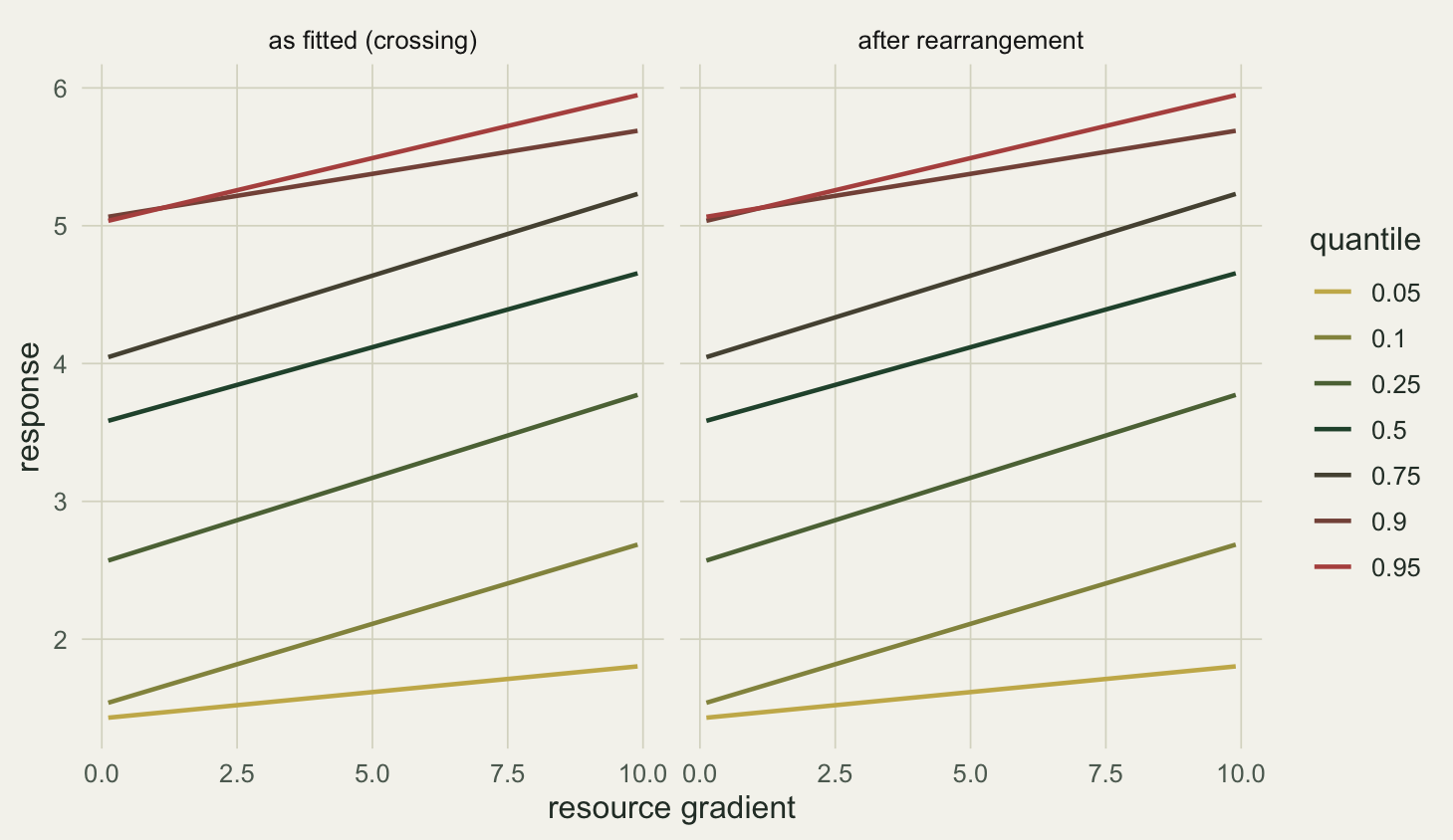
Each level is fitted on its own, so nothing forces the fitted lines to stay ordered. On a small sample with a near-flat slope, the noisy tail fits can invert, putting a lower-quantile line above a higher-quantile one over part of the range.

set.seed(4205)
n <- 50
x <- runif(n, 0, 10)
y <- 3 + 0.15 * x + rnorm(n, 0, 1.1)     # near-flat slope, homoscedastic
taus <- c(0.05, 0.1, 0.25, 0.5, 0.75, 0.9, 0.95)
co <- t(sapply(taus, function(t) qrfit(x, y, t)))
xg <- seq(min(x), max(x), length.out = 200)
Q  <- sapply(seq_along(taus), function(i) co[i, 1] + co[i, 2] * xg)
viol <- apply(Q, 1, function(r) any(diff(r) < 0))     # any inversion across levels
sum(viol)

[1] 21

Crossing occurs at 21 of the 200 grid positions, over x from 0.12 to 1.1, at the sparse lower edge where the extreme fits are least stable. The fix is rearrangement: at each value of x, sort the fitted quantiles into increasing order. The sorted curves are closer to the truth than the originals and cannot cross (Chernozhukov, Fernandez-Val and Galichon 2010).

Qr <- t(apply(Q, 1, sort))                 # monotone rearrangement at each x
sum(apply(Qr, 1, function(r) any(diff(r) < 0)))

[1] 0

After rearrangement the number of crossings is 0.

Figure 1: Independently fitted quantile lines cross at the sparse edge (left); rearrangement restores order (right).

Calibration is mechanical in sample

A tau fit places close to a fraction tau of the training points below it by construction. That number is not evidence of a good fit; it is a property of the check loss. The test is out of sample, and it is worth looking at it locally rather than only on average, because a wrong functional form can be right on average while being wrong region by region.

calib <- function(seed, curved, t = 0.9) {
  set.seed(seed)
  N <- 800; xx <- runif(N, 0, 10)
  mu <- if (curved) 6 * (1 - exp(-0.35 * xx)) else 1 + 0.4 * xx
  yy <- mu + rnorm(N, 0, 1)
  tr <- 1:400; te <- 401:N
  b  <- qrfit(xx[tr], yy[tr], t)
  pr <- function(idx) b[1] + b[2] * xx[idx]
  tc <- cut(xx[te], quantile(xx[te], c(0, 1/3, 2/3, 1)), include.lowest = TRUE,
            labels = c("low", "mid", "high"))
  c(train = mean(yy[tr] < pr(tr)), test = mean(yy[te] < pr(te)),
    tapply(yy[te] < pr(te), tc, mean))
}
rbind(well_specified = calib(4215, FALSE), misspecified = calib(4216, TRUE))

                train   test       low       mid      high
well_specified 0.9000 0.8750 0.8656716 0.8646617 0.8947368
misspecified   0.9025 0.9025 0.9179104 0.8270677 0.9624060

Both fits place 0.9 and 0.902 of the training points below the ninetieth-percentile line, matching the level as they must. Out of sample the well-specified fit stays near 0.9 everywhere. The misspecified fit, a straight line through a saturating truth, gives an out-of-sample proportion of 0.902, which looks fine. Split into thirds it is not: 0.918 in the low region, 0.827 in the middle and 0.962 at the top. The straight line under-covers where the curve bends away and over-covers where it flattens, and the two errors cancel in the average. Local calibration catches the misspecification that overall calibration hides.

The tail rests on a handful of points

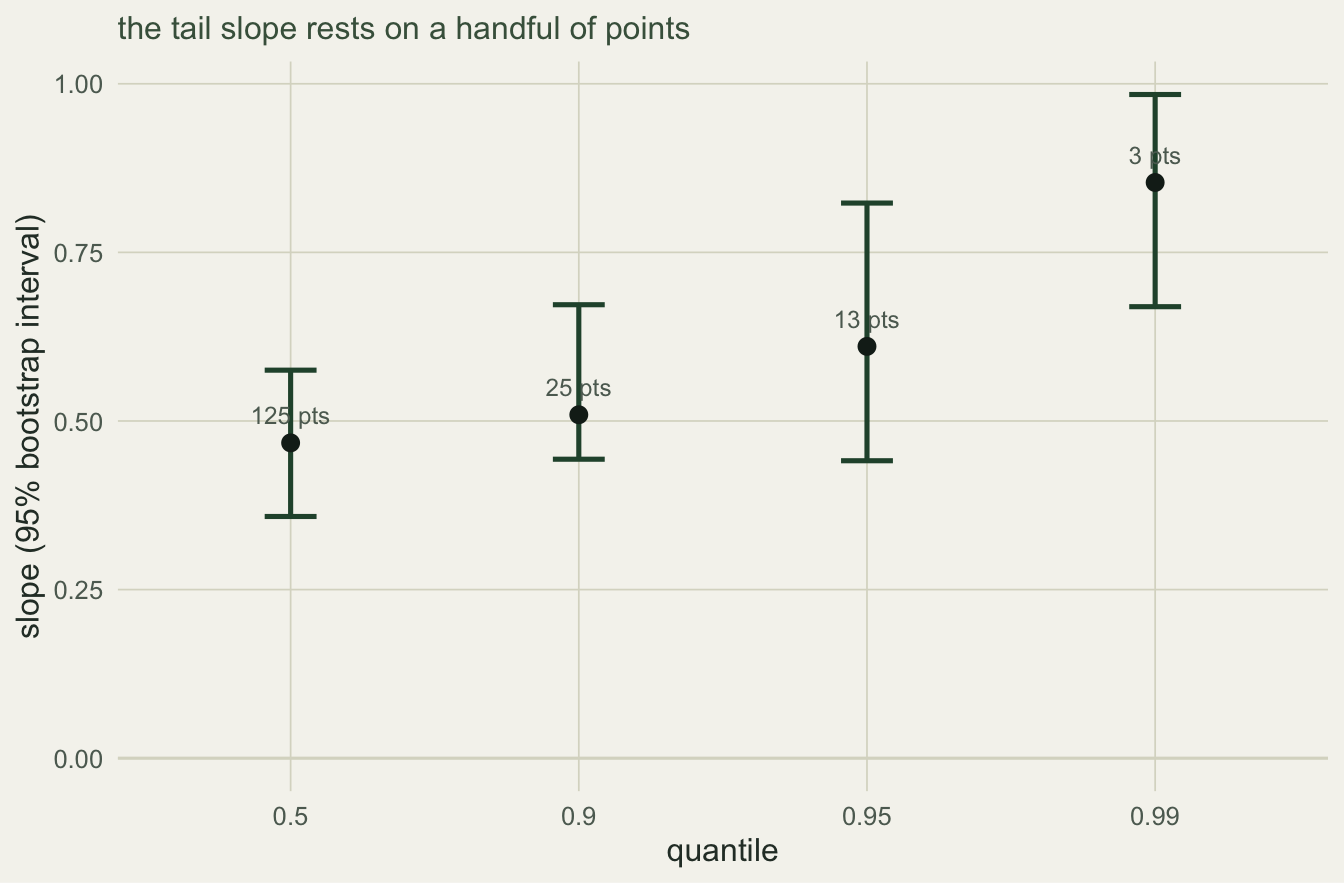
The asymptotic variance of a quantile estimate grows as the density at that quantile falls, so an extreme quantile is estimated from few points and its slope is far less certain than a central one. A bootstrap makes the growth visible.

set.seed(4225)
n2 <- 250
x2 <- runif(n2, 0, 10)
y2 <- 1 + 0.5 * x2 + rnorm(n2, 0, 1 + 0.12 * x2)   # unbounded, heteroscedastic tails
tset <- c(0.5, 0.9, 0.95, 0.99)
B <- 1000
set.seed(2020)
boot <- sapply(tset, function(t)
  replicate(B, { i <- sample(n2, n2, TRUE); qrfit(x2[i], y2[i], t)[2] }))
w <- apply(boot, 2, function(b) diff(quantile(b, c(.025, .975))))
data.frame(tau = tset, points_above = round(n2 * (1 - tset)), ci_width = round(w, 3))

   tau points_above ci_width
1 0.50          125    0.217
2 0.90           25    0.229
3 0.95           13    0.382
4 0.99            3    0.315

The width of the ninety-five per cent interval for the slope is 0.217 at the median but 0.382 at the ninety-fifth percentile, a factor of 1.76 wider, and the ninety-ninth percentile slope is determined by roughly three points, where the estimate jumps to 0.854 and its interval is both wide and unstable. There is no fix for this from within the data: a tail quantile needs tail observations, and if they are not there, no amount of computation supplies them.

Figure 2: Bootstrap slope estimate and interval by quantile level, with the number of points above each fitted line. The interval widens sharply into the tail.

The honest limit

The diagnostics constrain a quantile fit but do not vindicate it. Rearrangement removes crossing but does not make the sparse-edge fits trustworthy; it only enforces an ordering they should have had. Local calibration can reveal a wrong form but a passing check does not confirm the form is right, only that it was not caught. And the bootstrap interval on a tail slope describes the sampling variability of the sample-quantile relationship, not the distance from some true limiting relationship. The estimated tail slope is a function of the level you chose and the density of data in that tail, not a fact about the system. This is the same move that runs through the cluster and the wider blog: an E-value turns unmeasured confounding into a magnitude that would be needed, a delta adjustment turns an untestable missingness assumption into a tipping point, a reference frame turns a compositional claim into a total that would have to change. Here the level and the tail density are the knobs, and honest reporting means naming them rather than presenting a tail slope as settled.

References

Chernozhukov, Fernandez-Val and Galichon 2010 Econometrica 78(3):1093-1125 (10.3982/ECTA7880)

Koenker and Machado 1999 Journal of the American Statistical Association 94(448):1296-1310 (10.1080/01621459.1999.10473882)

Angrist, Chernozhukov and Fernandez-Val 2006 Econometrica 74(2):539-563 (10.1111/j.1468-0262.2006.00671.x)

Cade and Noon 2003 Frontiers in Ecology and the Environment 1(8):412-420 (10.1890/1540-9295(2003)001[0412:AGITQR]2.0.CO;2)

Koenker 2005 Quantile Regression, Cambridge University Press (ISBN 978-0-521-84573-1)

Related tutorials

• Quantile regression in ecology: beyond the mean
• Heteroscedasticity and limiting factors
• Distributional regression with location and scale
• Bootstrap confidence intervals