library(ggplot2)
library(patchwork)

te_paper  <- "#f5f4ee"
te_ink    <- "#16241d"
te_body   <- "#2c3a31"
te_forest <- "#275139"
te_rust   <- "#b5534e"
te_gold   <- "#c9b458"
te_line   <- "#dad9ca"

theme_datasheet <- function() {
  theme_minimal(base_size = 12) +
    theme(plot.background  = element_rect(fill = te_paper, colour = NA),
          panel.background = element_rect(fill = te_paper, colour = NA),
          panel.grid.major = element_line(colour = te_line, linewidth = 0.3),
          panel.grid.minor = element_blank(),
          text             = element_text(colour = te_body),
          plot.title       = element_text(colour = te_ink, face = "bold"),
          plot.subtitle    = element_text(colour = te_body),
          axis.text        = element_text(colour = te_body))
}Conditional simulation versus kriging
R
spatial
geostatistics
simulation
ecology tutorial
A kriged map is the best guess cell by cell but too smooth for the area above a threshold, the peak or the patch count. Conditional simulation in base R.
A restoration team has put eighty dipwells into a drained upland bog and read the water table in each of them. The target plant community needs ground that stays wet, and the team has turned that into a rule on a standardised scale: a cell counts as suitable when its water table sits more than one standard deviation above the long-run mean for the site, taken from the fitted model. The managers ask three questions. How much of the bog is suitable now, what is the wettest point, and is the suitable ground one block or a scatter of small pieces that a specialist invertebrate cannot move between? The analyst krigs the dipwells onto a grid, colours the cells above the threshold, and reads all three answers off the map.
The first two answers are biased, and so is the patch count behind the third, in a direction that can be predicted before the data arrive. The kriging tutorial on this site compares inverse distance weighting with ordinary kriging and closes the comparison of the two surfaces with the sentence “Both honour the data, but only one looks like a field.” That sentence is true of the comparison it makes: next to the bullseye halos of inverse distance weighting, the kriged surface has the coherent structure of a real field. It stays true for as long as the question is pointwise, a value at a cell with its standard error. It stops being true when the question is about the map as a whole, because the kriged surface is an average over every field consistent with the data, and an average of rough fields is smooth.
The variogram and GP kernel post showed that simple kriging and the Gaussian process posterior mean are the same predictor, and simulated its fields with a Cholesky factor written out by hand; this post uses the same construction. The Gaussian process regression post describes that posterior mean as a penalised smoother. The step neither post takes is to draw from the posterior instead of summarising it. On a map those draws are called conditional simulations: fields that pass through every dipwell and carry the roughness that the kriged surface averages away. The rest of the post measures, over sixty simulated surveys with a known truth, what the kriged map gets wrong about area, peak and patches, what the simulations get right, and the one comparison where kriging wins outright.
A bog, eighty dipwells and a known covariance
The field is a Gaussian random field on a square of side one, cut into a grid of 40 by 40 cells, with mean zero, variance one and an exponential covariance whose scale parameter is 0.15 of the side. Each survey places 80 dipwells in cells drawn at random and reads the field there without measurement error. The covariance, grid, dipwell count and threshold were set before the first run; only the number of surveys was raised, from forty to sixty, for Monte Carlo precision.
The covariance is treated as known. That removes variogram estimation from the comparison, which is a real simplification and returns in the limits section, but it isolates the question of the post: given the right model, what does the kriged map misrepresent? With a known mean and covariance the best linear predictor is simple kriging, and its weights and its variance take two lines. Conditional simulation uses the kriging residual construction that Journel set out in 1974, and that Journel and Huijbregts give in full in their textbook: simulate an unconditional field, krige the difference between the data and that field at the dipwells, and add the correction back. The result honours the data exactly and has the right conditional covariance everywhere else.
n_side    <- 40                      # cells along each side of the square
n_cell    <- n_side^2
cell_w    <- 1 / n_side
range_par <- 0.15                    # exponential covariance scale, side = 1
sill      <- 1                       # variance of the standardised field
n_obs     <- 80                      # dipwells per survey
thr_wet   <- 1                       # suitable ground: one sill sd above mean
n_sim     <- 200                     # conditional realisations per survey
n_truth   <- 60                      # independent simulated surveys

cell_xy  <- expand.grid(x = (seq_len(n_side) - 0.5) * cell_w,
                        y = (seq_len(n_side) - 0.5) * cell_w)
dist_mat <- as.matrix(dist(cell_xy))
cov_full <- sill * exp(-dist_mat / range_par)
chol_up  <- chol(cov_full)

krige_survey <- function(field, obs_id) {
  w_mat <- cov_full[, obs_id] %*% solve(cov_full[obs_id, obs_id])
  list(w_mat = w_mat,
       pred  = as.vector(w_mat %*% field[obs_id]),
       kvar  = sill - rowSums(w_mat * cov_full[, obs_id]))
}

cond_sims <- function(field, obs_id, w_mat, n_real) {
  unc <- crossprod(chol_up, matrix(rnorm(n_cell * n_real), n_cell, n_real))
  unc + w_mat %*% (field[obs_id] - unc[obs_id, , drop = FALSE])
}
A single survey first, so that the objects are visible before they are counted. One true field is drawn, one set of dipwells is placed, and the kriged map and two hundred conditional simulations are computed from the same dipwell values.
set.seed(2208)
truth_ex <- as.vector(crossprod(chol_up, rnorm(n_cell)))
obs_ex   <- sample.int(n_cell, n_obs)
kr_ex    <- krige_survey(truth_ex, obs_ex)
sim_ex   <- cond_sims(truth_ex, obs_ex, kr_ex$w_mat, n_sim)

data_gap_ex <- max(abs(kr_ex$pred[obs_ex] - truth_ex[obs_ex]),
                   abs(sim_ex[obs_ex, ] - truth_ex[obs_ex]))
sd_truth_ex <- sd(truth_ex)
sd_krig_ex  <- sd(kr_ex$pred)
sd_sim_ex   <- sd(sim_ex[, 1])
All four maps pass through the data: the largest discrepancy at a dipwell, over the kriged map and all 200 simulations, is 1.84e-14, which is rounding. They differ everywhere else. Across its cells the true field has a standard deviation of 0.923 in this survey and the first simulation 0.994; the kriged map has 0.817, and the figure shows where the difference goes. Between the dipwells the kriged surface relaxes towards the mean in broad pale saddles, while the true field and both simulations stay speckled at the scale of a few cells.
map_df <- rbind(
  data.frame(cell_xy, value = truth_ex,      panel = "true field"),
  data.frame(cell_xy, value = kr_ex$pred,    panel = "kriged map"),
  data.frame(cell_xy, value = sim_ex[, 1],   panel = "conditional simulation 1"),
  data.frame(cell_xy, value = sim_ex[, 2],   panel = "conditional simulation 2"))
map_df$panel <- factor(map_df$panel, levels = unique(map_df$panel))
well_df <- cell_xy[obs_ex, ]

ggplot(map_df, aes(x, y, fill = value)) +
  geom_raster() +
  geom_point(data = well_df, aes(x, y), inherit.aes = FALSE,
             shape = 21, fill = te_paper, colour = te_ink, size = 1.1, stroke = 0.3) +
  scale_fill_gradient2(low = te_gold, mid = te_paper, high = te_forest,
                       midpoint = 0, name = "standardised\nwater table") +
  facet_wrap(~ panel, ncol = 2) +
  coord_equal(expand = FALSE) +
  labs(x = NULL, y = NULL, title = "Four maps that agree at every dipwell",
       subtitle = "open circles: the eighty dipwells shared by all four panels") +
  theme_datasheet() +
  theme(axis.text = element_blank(), panel.grid.major = element_blank(),
        strip.text = element_text(colour = te_ink, face = "bold"))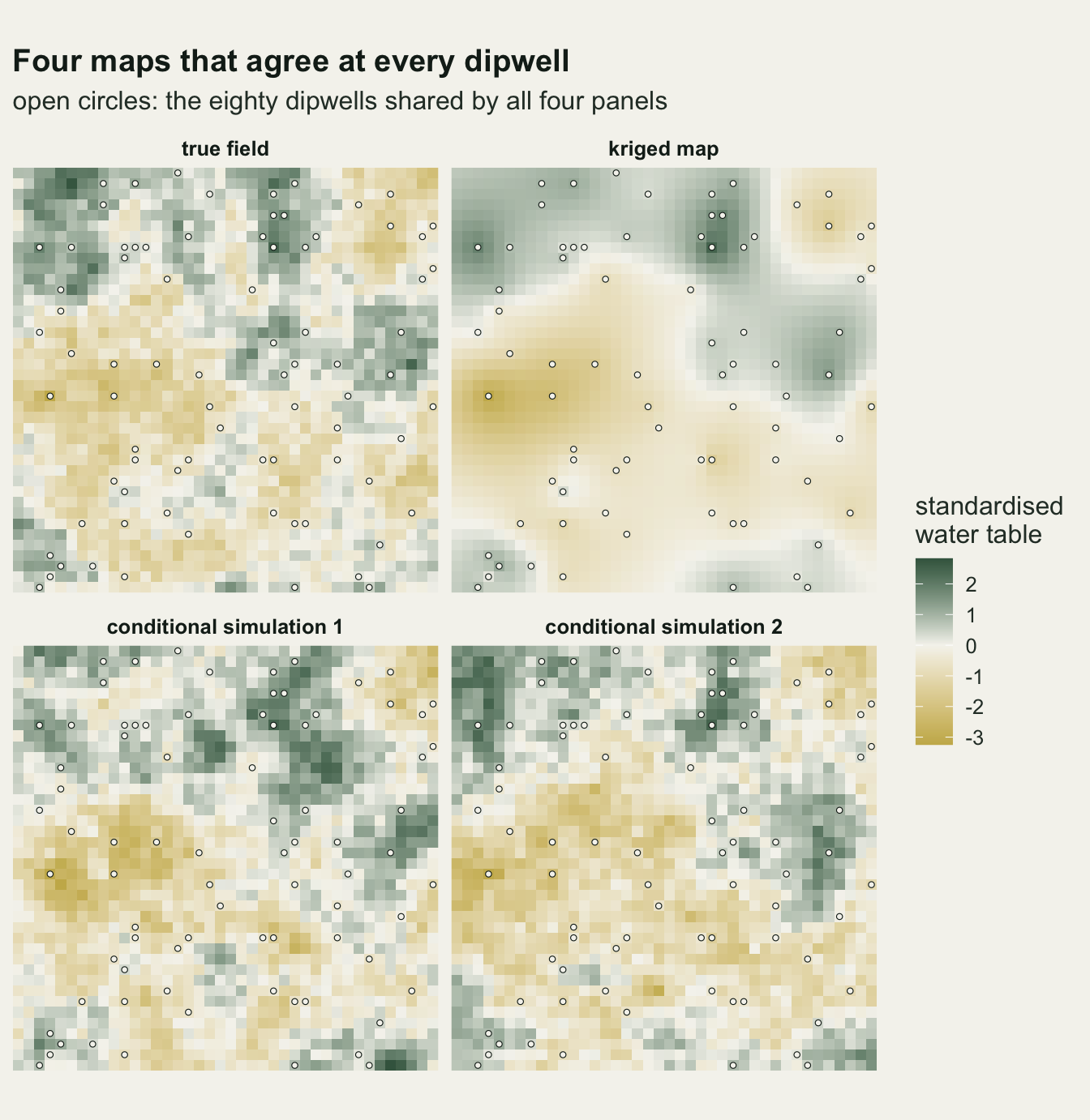
The kriged map is smoother than the field
The single map is an illustration. The comparison needs repetition, so the whole survey is run 60 times with a fresh true field and fresh dipwell positions each time, and every realisation of every survey is scored against its own truth. The patch counts use four neighbour connectivity on the grid. The labelling is done by repeated minimum filtering over all realisations of a survey at once, which is slow per step but needs no package.
thr_grid <- seq(-2, 2, by = 0.25)

label_patches <- function(ind_arr) {
  big <- n_cell + 1
  lab <- array(seq_len(n_cell), dim = dim(ind_arr))
  lab[!ind_arr] <- big
  rows_dn <- c(1, seq_len(n_side - 1)); rows_up <- c(2:n_side, n_side)
  repeat {
    old <- lab
    lab <- pmin(lab, lab[rows_up, , , drop = FALSE], lab[rows_dn, , , drop = FALSE],
                lab[, rows_up, , drop = FALSE], lab[, rows_dn, , drop = FALSE])
    lab[!ind_arr] <- big
    if (identical(lab, old)) break
  }
  apply(lab, 3, function(v) {
    v <- v[v < big]
    if (length(v) == 0) return(c(0, 0))
    tb <- tabulate(v)
    c(sum(tb > 0), max(tb))
  })
}

set.seed(5310)
study <- lapply(seq_len(n_truth), function(r) {
  truth  <- as.vector(crossprod(chol_up, rnorm(n_cell)))
  obs_id <- sample.int(n_cell, n_obs)
  kr     <- krige_survey(truth, obs_id)
  sims   <- cond_sims(truth, obs_id, kr$w_mat, n_sim)
  sim_mean <- rowMeans(sims)
  all_f  <- cbind(truth, kr$pred, sims)
  pat    <- label_patches(array(all_f > thr_wet, dim = c(n_side, n_side, ncol(all_f))))
  unobs  <- setdiff(seq_len(n_cell), obs_id)
  list(var_ratio = var(kr$pred) / var(truth),
       kvar_mean = mean(kr$kvar),
       spread_mean = mean(apply(sims, 1, var)),
       area_thr = rbind(truth = sapply(thr_grid, function(u) mean(truth > u)),
                        krig  = sapply(thr_grid, function(u) mean(kr$pred > u)),
                        sims  = sapply(thr_grid, function(u) mean(sims > u)),
                        avg   = sapply(thr_grid, function(u) mean(sim_mean > u))),
       area  = colMeans(all_f > thr_wet),
       peak  = apply(all_f, 2, max),
       well_max = max(truth[obs_id]),
       n_pat = pat[1, ], big_pat = pat[2, ],
       rmse  = c(krig = sqrt(mean((kr$pred - truth)[unobs]^2)),
                 one  = sqrt(mean((sims[unobs, 1] - truth[unobs])^2)),
                 avg  = sqrt(mean((sim_mean - truth)[unobs]^2))))
})
pull <- function(nm) sapply(study, `[[`, nm)
var_ratio <- pull("var_ratio")
vr_mean <- mean(var_ratio)
vr_se <- sd(var_ratio) / sqrt(n_truth)
kvar_all <- mean(pull("kvar_mean"))
spread_all <- mean(pull("spread_mean"))
marg_krig <- sill - kvar_allOver the 60 surveys, the variance of the kriged map across its own cells is 0.574 of the variance of the true field across the same cells, with a standard error of 0.013 between surveys. How much is lost depends on the design: more dipwells or a longer correlation range would raise the ratio, and sparser sampling would lower it.
The ratio is not a quirk of the simulation. At any cell the true value is the kriged value plus an error that is uncorrelated with it, so the variance of the field splits into the variance of the prediction and the kriging variance, and the prediction can only keep what the error does not take. The mean kriging variance over all cells and surveys is 0.399, which leaves 0.601 of the sill for the prediction. The within map ratio sits a little below that, because both the field and the kriged map lose the part of their variation that is shared by the whole square, and that shared part is the part the dipwells pin down best. On average the kriged map carries a little under three fifths of the variability of the thing it maps. The kriging variance itself does not depend on the values read, only on the design and the covariance, but a single survey can lose much more or much less: the ratio ranged from 0.36 to 0.84 across the sixty surveys.
Simulations put the variance back, one map at a time
A conditional simulation is the kriged value plus a draw of the missing error, so the spread of the simulations at a cell should reproduce the kriging variance. Over all cells and surveys the variance between simulations averages 0.400 against a mean kriging variance of 0.399. The simulations put back the variance that the prediction lacks, and they put back the right amount.
That cannot come for free, and the price is paid in pointwise accuracy. A simulated value and the true value are two independent draws from the same conditional distribution, so the squared error of one simulation at a cell has twice the expected size of the kriging error, and its root mean squared error should be larger by the square root of two.
rmse_tab  <- pull("rmse")
rmse_krig <- mean(rmse_tab["krig", ])
rmse_one  <- mean(rmse_tab["one", ])
rmse_avg  <- mean(rmse_tab["avg", ])
rmse_ratio <- rmse_one / rmse_krig
one_worse  <- mean(rmse_tab["one", ] > rmse_tab["krig", ])
Scored on the cells without a dipwell, the kriged map has a root mean squared error of 0.643 and a single conditional simulation 0.904, a ratio of 1.407 against the square root of two, 1.414. The single simulation was the worse pointwise map in 100 per cent of the 60 surveys. Averaging the 200 simulations cell by cell gives back an error of 0.645, the kriging figure plus a little Monte Carlo noise, because the average of the conditional distribution is the kriged value.
So the claim that a simulation is a better map is false in the sense that most readers would test first. As a cell by cell guess, kriging is better than any one realisation, and the realisations only match it again when they are averaged into it. What the realisations have that the average does not is the joint behaviour of many cells at once, and every question the bog managers asked is of that kind.
Area above a threshold
The fraction of the area above the threshold is a count of cells, and whether a cell is counted depends on its value in a way that is not linear. Replacing each value by its conditional mean before counting is therefore not the same as counting in each plausible field and then averaging the count. The threshold of one standard deviation sits above the mean, so a map that has been pulled towards the mean will cross it in fewer cells. The same sweep was run over thresholds from minus two to plus two to see the whole pattern.
area_mat  <- pull("area")
area_true <- area_mat[1, ]
area_krig <- area_mat[2, ]
area_sims <- area_mat[-(1:2), , drop = FALSE]
area_simm <- colMeans(area_sims)
area_lo   <- apply(area_sims, 2, quantile, probs = 0.05)
area_hi   <- apply(area_sims, 2, quantile, probs = 0.95)

rel_bias <- function(est, tru) {
  d_vec <- est - tru
  c(bias = 100 * mean(d_vec) / mean(tru),
    se   = 100 * sd(d_vec) / sqrt(n_truth) / mean(tru))
}
bias_area_k <- rel_bias(area_krig, area_true)
bias_area_s <- rel_bias(area_simm, area_true)
cover_area  <- mean(area_true >= area_lo & area_true <= area_hi)
cover_se    <- sqrt(0.9 * 0.1 / n_truth)
krig_below  <- mean(area_krig < area_true)
mean_area_t <- mean(area_true)
thr_idx     <- which(thr_grid == thr_wet)

thr_arr  <- simplify2array(lapply(study, `[[`, "area_thr"))
dimnames(thr_arr)[[1]] <- c("truth", "krig", "sims", "avg")
thr_mean <- apply(thr_arr, c(1, 2), mean)
avg_area_ratio <- thr_mean["avg", thr_idx] / thr_mean["truth", thr_idx]
thr_lo_idx <- which(thr_grid == -thr_wet)
krig_over_lo <- 100 * (thr_mean["krig", thr_lo_idx] / thr_mean["truth", thr_lo_idx] - 1)
At the threshold, the true fraction of suitable ground averages 0.148 over the surveys. The kriged map estimates it with a relative bias of -36.6 per cent (standard error 2.2), and it came in below the truth in 100 per cent of surveys, so this is not a matter of an unlucky site. The mean of the per realisation areas has a relative bias of +3.1 per cent with a standard error of 1.6. That is a distance of 1.9 standard errors from zero. The simulation is exact for the model that generated the data, so its expected bias is zero, and a departure of that size is consistent with Monte Carlo noise from sixty surveys.
The route matters as much as the tool. Average the simulations cell by cell first and then count, and the area comes out at 0.634 of the truth, no better than kriging, because that average is the kriged map again.
thr_df <- data.frame(threshold = rep(thr_grid, each = 4),
                     map = rep(c("true field", "kriged map", "conditional simulations",
                                 "average of the simulations"), length(thr_grid)),
                     area = as.vector(thr_mean))
thr_df$map <- factor(thr_df$map, levels = c("true field", "conditional simulations",
                                            "kriged map", "average of the simulations"))

ggplot(thr_df, aes(threshold, area, colour = map, linetype = map)) +
  geom_vline(xintercept = thr_wet, colour = te_body, linetype = "dotted", linewidth = 0.6) +
  geom_line(linewidth = 0.9) +
  scale_colour_manual(values = c(te_ink, te_gold, te_forest, te_rust), name = NULL) +
  scale_linetype_manual(values = c("solid", "dashed", "solid", "dotdash"), name = NULL) +
  labs(x = "threshold (standardised water table)", y = "fraction of the area above",
       title = "The smooth map misses both tails",
       subtitle = "dotted line: the threshold for suitable ground") +
  guides(colour = guide_legend(nrow = 2), linetype = guide_legend(nrow = 2)) +
  theme_datasheet() +
  theme(legend.position = "bottom", legend.key.width = unit(2.2, "lines"))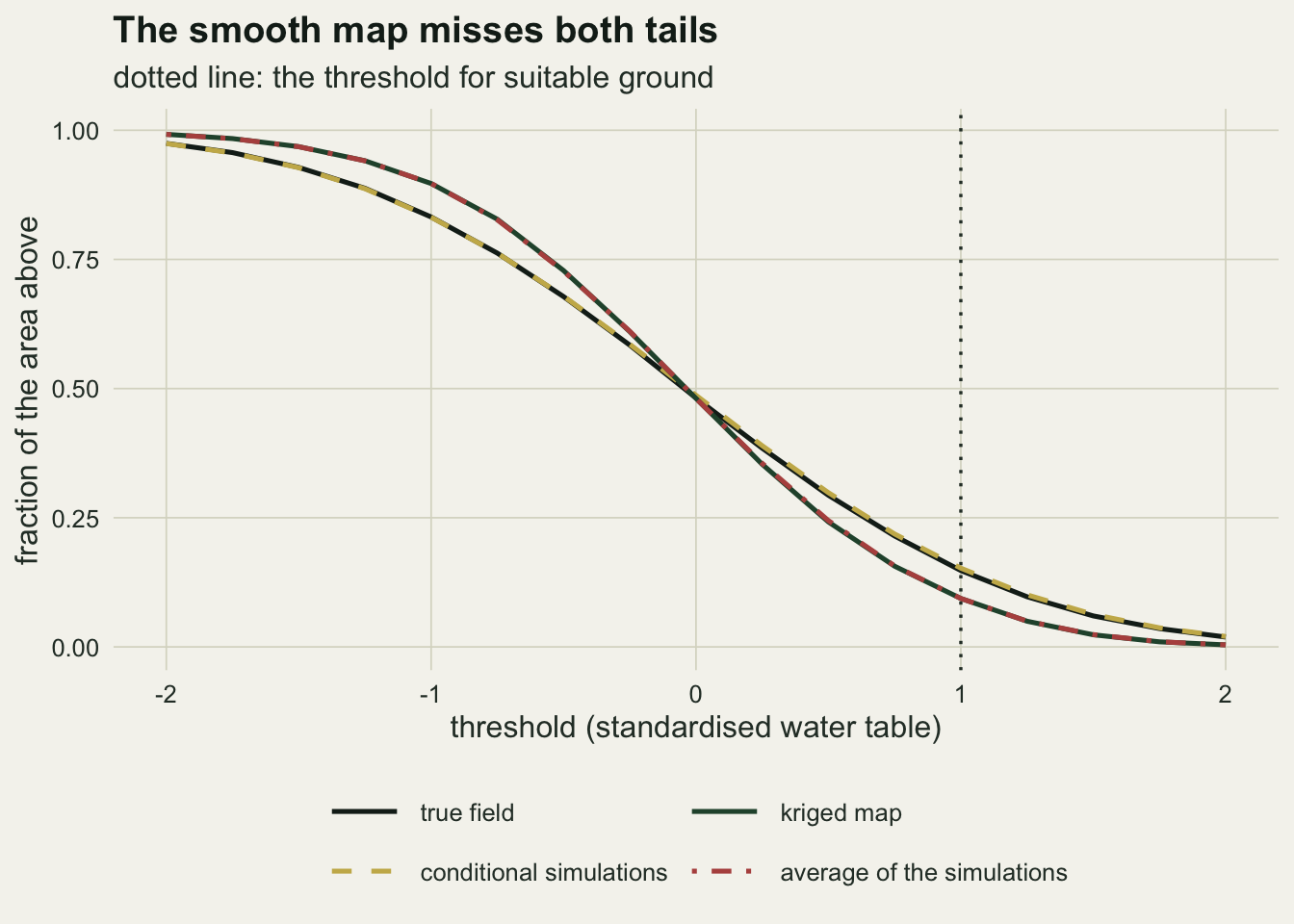
The threshold sweep shows the bias changing sign with the side of the mean. Below the mean the smooth map has too few cells in the lower tail, so it overstates the area above the threshold instead: at minus one the kriged fraction is +7.8 per cent against the truth. Near zero, where the threshold cuts the distribution through its middle, the curves meet. An area of suitable habitat defined by an upper threshold is understated, and an area defined by a lower one, such as ground dry enough for a nesting wader, is overstated. A relative bias also grows as the threshold moves into the upper tail, since the true area shrinks faster than the absolute error does.
The simulations also give each survey an uncertainty statement for the area itself, which the kriged map has no way to produce: a kriging standard error belongs to a cell, not to a count of cells. The central 90 per cent interval of the 200 simulated areas contained the true area in 95 per cent of surveys, with a Monte Carlo standard error of 3.9 percentage points on that rate.
area_df <- data.frame(true_area = area_true, krig = area_krig, simm = area_simm,
                      lo = area_lo, hi = area_hi)
lim_area <- c(0, max(c(area_df$hi, area_df$true_area)) * 1.02)

p_krig <- ggplot(area_df, aes(true_area, krig)) +
  geom_abline(slope = 1, intercept = 0, colour = te_body, linetype = "dashed") +
  geom_point(colour = te_forest, size = 2) +
  coord_equal(xlim = lim_area, ylim = lim_area) +
  labs(x = "true fraction above threshold", y = "estimated fraction",
       title = "Kriged map") +
  theme_datasheet()

p_sims <- ggplot(area_df, aes(true_area, simm)) +
  geom_abline(slope = 1, intercept = 0, colour = te_body, linetype = "dashed") +
  geom_errorbar(aes(ymin = lo, ymax = hi), colour = te_gold, width = 0, linewidth = 0.5) +
  geom_point(colour = te_ink, size = 2) +
  coord_equal(xlim = lim_area, ylim = lim_area) +
  labs(x = "true fraction above threshold", y = NULL,
       title = "Conditional simulations") +
  theme_datasheet()

p_krig + p_sims +
  plot_annotation(theme = theme(plot.background = element_rect(fill = te_paper, colour = NA)))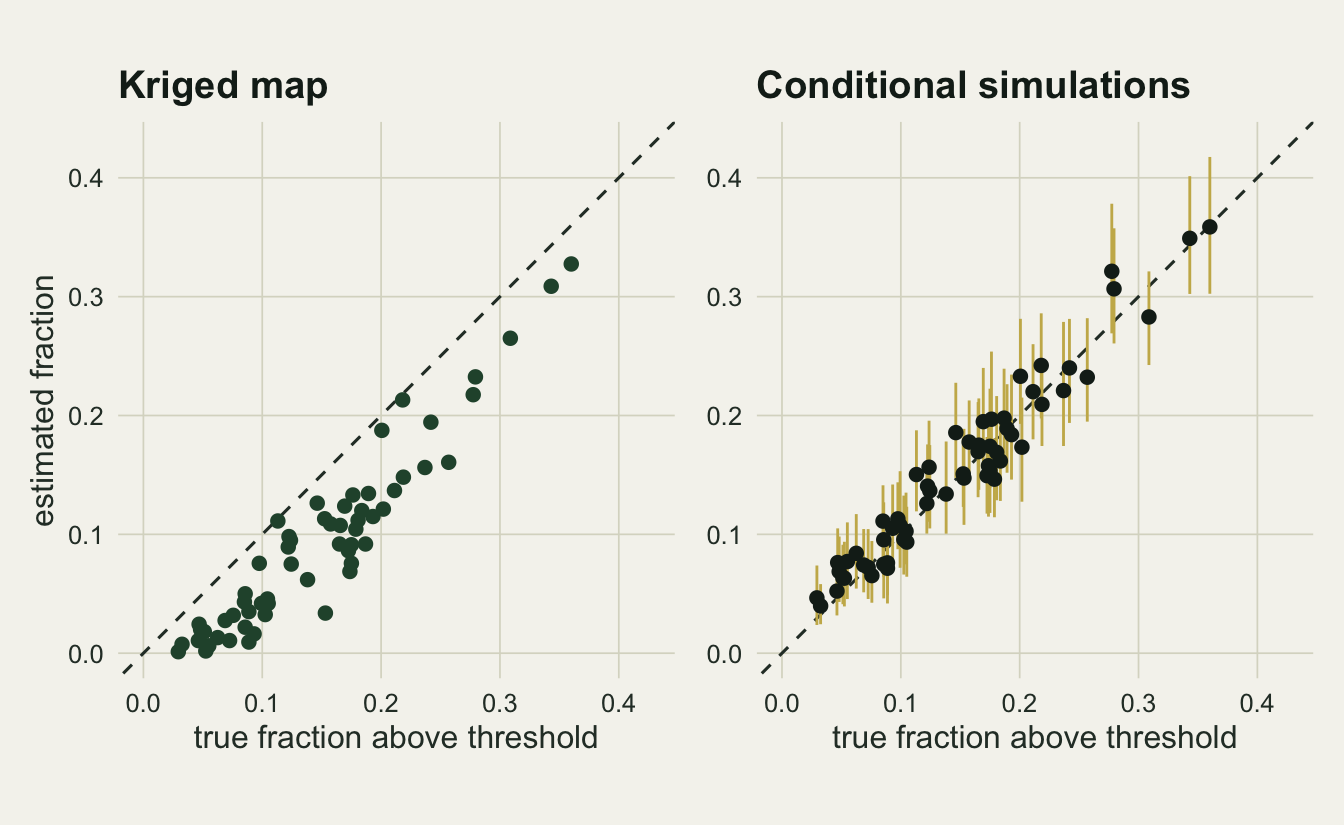
The peak and the patches
The wettest point and the number of separate wet patches are the other two questions. Both are further from linear than an area is. The maximum is decided by the one cell that happens to be highest, and a smooth map has no single high cell away from the dipwells; the patch count depends on whether neighbouring cells above the threshold touch.
peak_mat  <- pull("peak")
peak_true   <- mean(peak_mat[1, ])
peak_krig   <- mean(peak_mat[2, ])
well_mat    <- pull("well_max")
peak_at_well <- mean(abs(peak_mat[2, ] - well_mat) < 1e-8)
peak_true_minus_well <- mean(peak_mat[1, ] - well_mat)
gap_peak_k <- peak_mat[2, ] - peak_mat[1, ]
gap_peak_s <- colMeans(peak_mat[-(1:2), , drop = FALSE]) - peak_mat[1, ]
sd_units <- function(d_vec) c(bias = mean(d_vec), se = sd(d_vec) / sqrt(n_truth))
bias_peak_k <- sd_units(gap_peak_k)
bias_peak_s <- sd_units(gap_peak_s)

npat_mat <- pull("n_pat")
npat_true <- mean(npat_mat[1, ])
npat_krig <- mean(npat_mat[2, ])
npat_simm <- mean(colMeans(npat_mat[-(1:2), , drop = FALSE]))
bias_npat_s <- rel_bias(colMeans(npat_mat[-(1:2), , drop = FALSE]), npat_mat[1, ])
npat_fold   <- npat_true / npat_krig
npat_lo <- apply(npat_mat[-(1:2), , drop = FALSE], 2, quantile, probs = 0.05)
npat_hi <- apply(npat_mat[-(1:2), , drop = FALSE], 2, quantile, probs = 0.95)
cover_npat <- mean(npat_mat[1, ] >= npat_lo & npat_mat[1, ] <= npat_hi)

big_mat  <- pull("big_pat")
bias_big_k <- rel_bias(big_mat[2, ], big_mat[1, ])
bias_big_s <- rel_bias(colMeans(big_mat[-(1:2), , drop = FALSE]), big_mat[1, ])
big_true <- mean(big_mat[1, ])
The true peak of the standardised field averages 2.90 over the surveys and the kriged peak 2.16, so the kriged peak is lower by 0.74 standard deviations of the field (standard error 0.04). The mean simulated peak differs from the true peak by -0.01 standard deviations (standard error 0.04). The peak is given in standard deviations rather than per cent because its zero is the field mean, which is an arbitrary origin for a water table. Between dipwells the kriged surface bends back towards the mean, and in 100 per cent of surveys the kriged peak was exactly the highest dipwell reading, to rounding. The true peak lay above that reading by 0.74 on average, somewhere nobody had put a dipwell.
The patch count is where the kriged map fails worst. The true field has 28.6 separate patches above the threshold on average and the kriged map 4.5, so the truth holds 6.4 times as many. The mean over simulations is 29.7, a relative bias of +4.0 per cent with a standard error of 2.3, and the 90 per cent simulation interval contained the true count in 93 per cent of surveys.
npat_df <- data.frame(survey = rep(seq_len(n_truth), 3),
                      map = rep(c("true field", "kriged map", "mean of simulations"),
                                each = n_truth),
                      patches = c(npat_mat[1, ], npat_mat[2, ],
                                  colMeans(npat_mat[-(1:2), , drop = FALSE])))
npat_df$map <- factor(npat_df$map, levels = c("kriged map", "mean of simulations",
                                              "true field"))

ggplot(npat_df, aes(patches, map, colour = map)) +
  geom_jitter(height = 0.18, width = 0, size = 1.9, alpha = 0.8) +
  stat_summary(fun = mean, geom = "point", shape = 124, size = 9, colour = te_ink) +
  scale_colour_manual(values = c(te_forest, te_gold, te_rust), guide = "none") +
  labs(x = "separate patches above the threshold", y = NULL,
       title = "The kriged map loses the patches",
       subtitle = "one point per survey; vertical bar: the mean over sixty surveys") +
  theme_datasheet()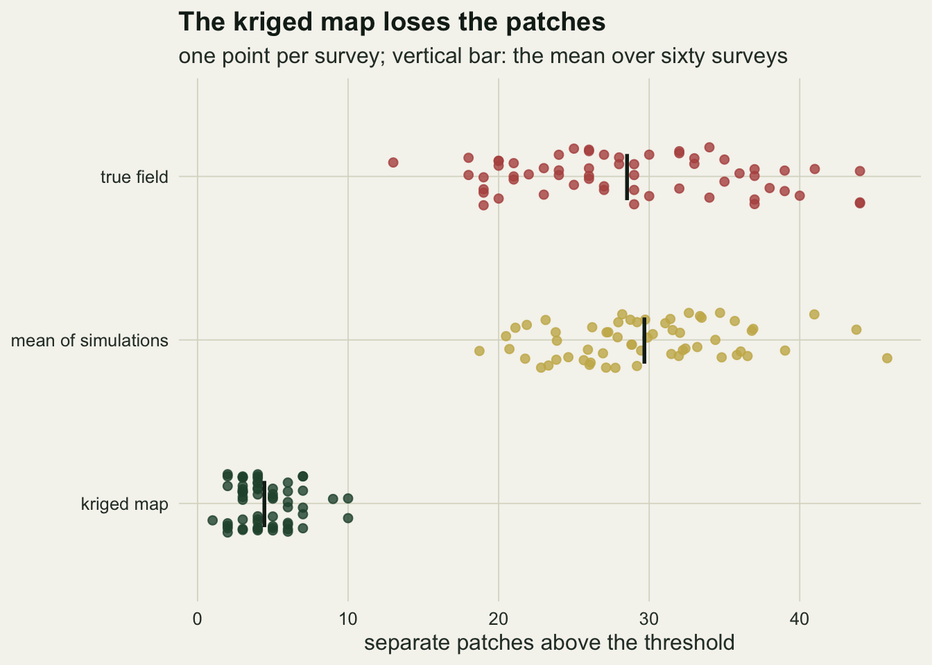
The size of the largest patch was measured too, and it does not follow the pattern. The kriged map’s largest patch has a relative bias of +6.3 per cent against a true mean of 96 cells, with a standard error of 7.4, and the simulation mean +11.9 per cent with a standard error of 6.3. Neither is clearly separated from zero with sixty surveys. On the kriged map the small patches vanish because too few cells cross the threshold, but the main wet block is where dipwells read high values and the surface stays above the threshold between them, so its extent is roughly kept. The statement that smoothing biases every connectivity measure is too strong: it removed the small patches here and left the largest one roughly intact, and a measure built on the small patches, such as the number of stepping stones, inherits the first failure.
What to report
Use the kriged map, with its standard error map, for any question asked of one location at a time: the expected water table at a proposed planting cell, or where a new dipwell would reduce uncertainty most. In the surveys above it had a lower pointwise error than a single simulation in 100 per cent of cases, and the simulations only equal it once they are averaged back into it.
Goovaerts made this argument for soil maps in 2001, and it applies unchanged to habitat maps. For any quantity computed from many cells together, compute it in each conditional simulation and report the mean and a percentile interval over realisations. That covers areas above or below a threshold, maxima and minima, patch counts, the length of a wet corridor, and totals passed through a nonlinear function such as a habitat suitability curve. Say which threshold was used and on which side of the mean it lies, because the direction of the kriging bias depends on it.
Report the number of realisations and the covariance model the simulations came from, including whether its parameters were estimated or fixed. A set of simulations is exactly as good as the variogram behind it, and with 200 realisations each end of a 90 per cent interval rests on the 10 most extreme realisations.
Do not publish a single simulation as the map. It honours the data and looks like a field, which makes it persuasive, and it has the larger pointwise error by a factor near the square root of two. Where a figure needs to show what the field could look like, show two or three realisations next to the kriged map, as in the first figure.
Honest limits
The covariance was known exactly and the mean was known to be zero. In real surveys the variogram is estimated, and ordinary or universal kriging replaces simple kriging; the simulations then inherit any error in the fitted range and sill, and plug-in simulations understate the uncertainty because they treat estimated parameters as fixed. A range fitted too long makes every realisation too smooth, and the patch counts above would be biased again in the kriging direction, by an amount this post did not measure.
The field was Gaussian and the threshold was applied to the field itself. Water table depth can be skewed, and a transformed field needs a back transformation in each realisation before the threshold is applied. Categorical or strongly non Gaussian variables need other simulation algorithms (indicator or truncated Gaussian simulation) that are not shown here.
The dipwells had no measurement error. With a nugget or a measurement variance, the kriged surface no longer passes through the data, the simulations must add a noise term to be comparable with readings, and the choice of whether the threshold applies to the underlying process or to a noisy reading becomes a real modelling decision.
Cholesky factorisation of the full 1600 by 1600 covariance is what made this cheap. The cost grows with the cube of the number of cells, so a real habitat map of a hundred thousand cells needs sequential Gaussian simulation, spectral methods or a sparse approximation; Chiles and Delfiner cover the algorithms and their trade offs. The results above do not depend on the algorithm, only on drawing from the correct conditional distribution.
The patch results depend on the grid. A finer grid, or eight neighbour connectivity, produces different counts in both the truth and the simulations, and patch counts are only comparable between maps drawn at the same resolution with the same rule. The exponential covariance also makes the field rough at the cell scale; a smoother covariance, such as a Gaussian or a Matern with larger smoothness, would change the gap between the kriged and true patch counts by an amount not measured here.
Sixty surveys give a clear answer on the large biases and a vague one on the small ones. The simulation means for area and patch count sit within about two standard errors of the truth, which is consistent with the zero bias that theory guarantees, but these runs could not detect a bias of a few per cent on their own.
References
Journel AG 1974 Economic Geology 69(5):673-687 (10.2113/gsecongeo.69.5.673)
Journel AG, Huijbregts CJ 1978 Mining Geostatistics (ISBN 0-12-391050-1)
Chiles J-P, Delfiner P 2012 Geostatistics: Modeling Spatial Uncertainty, 2nd edition (ISBN 978-0-470-18315-1)
Goovaerts P 2001 Geoderma 103(1-2):3-26 (10.1016/S0016-7061(01)00067-2)