library(ggplot2)

te_pal <- list(forest = "#275139", green = "#2f8f63", sage = "#93a87f",
               clay = "#b5534e", gold = "#cda23f", line = "#dad9ca",
               ink = "#16241d", paper = "#f5f4ee")

theme_te <- function() {
  theme_minimal(base_size = 12) +
    theme(panel.grid.minor = element_blank(),
          panel.grid.major = element_line(colour = "#e7e6dc"),
          plot.background = element_rect(fill = "#f5f4ee", colour = NA),
          panel.background = element_rect(fill = "#f5f4ee", colour = NA),
          plot.title = element_text(face = "bold", colour = te_pal$ink),
          axis.title = element_text(colour = "#2c3a31"),
          axis.text = element_text(colour = "#2c3a31"),
          legend.position = "bottom")
}Stream networks and tail-up covariance
R
spatial
GLS
freshwater
ecology tutorial
Stream distance is not Euclidean distance. Build a dendritic network in R, watch the Gaussian covariance fail, and fit a tail-up model and kriging by hand.
A fisheries team leaves forty-eight temperature loggers in a fifth-order catchment from June to August and gets back one mean summer temperature per site. The catchment drains about a hundred and twenty square kilometres through roughly a hundred kilometres of mapped channel, so the loggers sit on a small part of it. The question the team has is not about the forty-eight numbers. It is about the reaches with no logger, because that is where a thermal refuge either exists or does not, and a map is what the decision needs.
That is an interpolation problem, and this blog has a lot of machinery for interpolation. All of it assumes a plane. Distance between two points is the length of the straight line joining them; a kernel or a variogram turns that length into a correlation; kriging turns the correlations into a weighted average. Running water is not a plane. Two loggers two hundred metres apart across a watershed divide are, for anything that drifts, swims or dissolves, much further apart than two loggers twenty kilometres apart on the same channel. Worse, the pair on opposite sides of the divide are not merely far apart: nothing flows from either one to the other, and the covariance between them is a different kind of object from the covariance between two sites on the same thread of water.
Two neighbouring posts frame what follows. Isolation by distance and by resistance also measures a gap between straight-line distance and a better distance, and its finding is stated in a sentence worth quoting: fitting on Euclidean distance “leaves the barrier pairs 0.0093 above the line on average and the same-side pairs 0.0108 below it, a systematic offset in opposite directions for the two groups, which is what a missing predictor leaves behind.” The geometry there is still a plane, though. The alternative distance is a cost accumulated over a raster, every pair of sites has one, and the correction is a better horizontal axis for the same regression. Here the geometry itself is a tree, and the pairs split into two classes with no analogue on a plane: one site is downstream of the other, or neither is.
The second is generalised least squares for spatial data, which is where the correlation structures live. It closes its model-selection section with advice that this post is going to contradict, so it is worth having the exact words: “the decision that matters is whether to model spatial correlation, not which decay shape you choose; pick the best by AIC, but do not agonise between exponential and spherical when they tie.” On a plane that is correct, and nothing below overturns it there. On a network the choice of decay shape stops being cosmetic, for a reason that has nothing to do with fit.
Four things get measured. How far stream distance and Euclidean distance diverge, and how differently they diverge for the two classes of pair. What happens to the three standard correlation functions when stream distance is substituted for Euclidean distance in them. How a tail-up covariance is built from a moving average so that it is valid by construction, and how much the weighting rule at confluences matters. And what the wrong geometry costs in hold-out prediction and in the number a reader takes away as “the range”.
Everything is base R and ggplot2. The network, the distances, the covariance matrices, the restricted likelihood and the kriging predictor are all built here rather than called, which for a network is the more honest way round: on a real catchment the hard part is not the statistics but getting a digital stream layer into a topologically correct form, and that part is not simulated here. The packages that do it appear once, in a block that does not run.
A network is a parent pointer and a length
A stream network needs three things and no more: a set of nodes, one parent pointer per node saying which node the water goes to next, and a length for the segment between a node and its parent. Everything else, the drainage direction, the confluences, the headwaters, the notion of upstream, follows from those. The builder below grows a dendritic network from the outlet upwards. Each branch runs for a jittered length, is cut into three pieces so there are intermediate nodes to put loggers on, and then forks into two. Five levels of forking give a network of the size a small monitoring programme would cover.
build_network <- function(n_level, len0, shrink, spread, n_piece, seed) {
  set.seed(seed)
  nx <- 0; ny <- 0; np <- NA_integer_
  q_node <- 1L; q_ang <- pi / 2; q_lev <- 0L
  while (length(q_node) > 0) {
    nid <- q_node[1]; ang <- q_ang[1]; lev <- q_lev[1]
    q_node <- q_node[-1]; q_ang <- q_ang[-1]; q_lev <- q_lev[-1]
    blen <- len0 * shrink^lev * runif(1, 0.75, 1.25)
    cur <- nid
    for (k in seq_len(n_piece)) {
      ang <- ang + rnorm(1, 0, 0.18)
      nx <- c(nx, nx[cur] + (blen / n_piece) * cos(ang))
      ny <- c(ny, ny[cur] + (blen / n_piece) * sin(ang))
      np <- c(np, cur)
      cur <- length(nx)
    }
    if (lev + 1 < n_level) {
      for (s in c(-1, 1)) {
        q_node <- c(q_node, cur)
        q_ang <- c(q_ang, ang + s * spread * runif(1, 0.7, 1.3))
        q_lev <- c(q_lev, lev + 1L)
      }
    }
  }
  data.frame(id = seq_along(nx), parent = np, x = nx, y = ny)
}

net <- build_network(n_level = 5, len0 = 10, shrink = 0.68, spread = 0.62,
                     n_piece = 3, seed = 19)
n_node <- nrow(net)
seg_len <- sqrt((net$x - net$x[net$parent])^2 + (net$y - net$y[net$parent])^2)
seg_len[is.na(seg_len)] <- 0
n_child <- tabulate(net$parent[!is.na(net$parent)], nbins = n_node)
head_tip <- which(n_child == 0)

strahler <- integer(n_node)
for (i in rev(seq_len(n_node))) {
  ch <- which(net$parent == i)
  if (length(ch) == 0) strahler[i] <- 1L
  else strahler[i] <- if (sum(strahler[ch] == max(strahler[ch])) > 1)
    max(strahler[ch]) + 1L else max(strahler[ch])
}
print(c(nodes = n_node, confluences = sum(n_child > 1), headwaters = length(head_tip),
        stream_order_at_outlet = strahler[1]))
nodes confluences headwaters
94 15 16
stream_order_at_outlet
5 print(round(c(channel_km = sum(seg_len), width_km = diff(range(net$x)),
height_km = diff(range(net$y))), 3))channel_km width_km height_km
104.611 31.404 21.521 The result is 94 nodes, 15 confluences and 16 headwaters, 104.6 km of channel draining a box roughly 31 by 22 km, and a Strahler order of 5 at the outlet.
Stream distance now comes from two passes over the tree. The first accumulates, for every node, the channel distance down to the outlet and the list of nodes it passes through on the way. The second uses those lists: the common junction of two nodes is the first node that appears in both downstream paths, and the stream distance between them is the sum of their outlet distances minus twice the outlet distance of that junction.
out_dist <- numeric(n_node)
down_path <- vector("list", n_node)
for (i in seq_len(n_node)) {
  p <- net$parent[i]
  if (is.na(p)) {
    out_dist[i] <- 0
    down_path[[i]] <- integer(0)
  } else {
    out_dist[i] <- out_dist[p] + seg_len[i]
    down_path[[i]] <- c(p, down_path[[p]])
  }
}

common_junction <- function(i, j) {
  a <- c(i, down_path[[i]])
  b <- c(j, down_path[[j]])
  a[a %in% b][1]
}
print(round(c(outlet_distance_max = max(out_dist),
              headwater_min = min(out_dist[head_tip])), 3))
outlet_distance_max headwater_min
26.806 24.171 Two sites are flow-connected when one of them is their common junction, that is, when the water leaving the upper one passes the lower one. Otherwise they are flow-unconnected: they share a junction somewhere downstream, but neither drains into the other. Forty-eight nodes are drawn as logger positions, and the two distance matrices and the connection classes are built for all pairs.
set.seed(101)
site_id <- sort(sample(2:n_node, 48))
n_site <- length(site_id)
junc <- outer(site_id, site_id, Vectorize(common_junction))
str_d <- outer(out_dist[site_id], out_dist[site_id], "+") - 2 * out_dist[junc]
conn <- (junc == site_id) | (junc == matrix(site_id, n_site, n_site, byrow = TRUE))
euc_d <- as.matrix(dist(net[site_id, c("x", "y")]))
up_tri <- upper.tri(str_d)

n_pair <- sum(up_tri)
n_conn <- sum(conn[up_tri])
print(c(sites = n_site, pairs = n_pair, flow_connected = n_conn,
        flow_unconnected = n_pair - n_conn))
sites pairs flow_connected flow_unconnected
48 1128 218 910 print(round(c(max_stream_km = max(str_d), max_euclid_km = max(euc_d)), 3))max_stream_km max_euclid_km
37.030 30.603 Of the 1128 pairs, 218 are flow-connected and 910 are not, so four pairs in five are of the kind that a planar model has no name for. That ratio is a property of tree geometry rather than of this particular tree: a site is flow-connected only to the sites on its own thread down to the outlet and the sites upstream of it, which is a thin slice of a branching network.
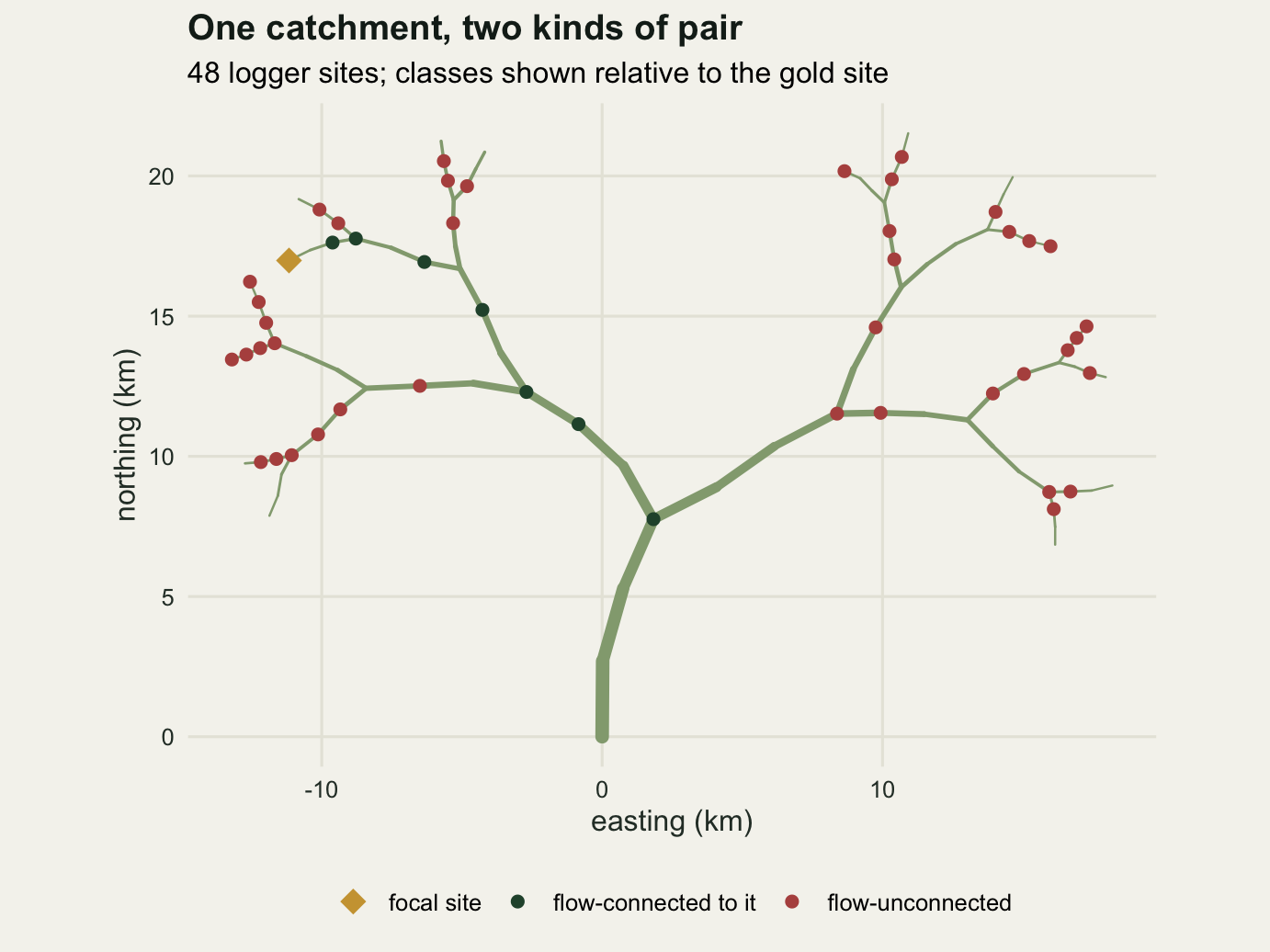
Two distances, and the class that has no planar analogue
The comparison to run is the one the resistance post ran: put the two distances against each other and see where they disagree. The difference is that here the pairs come pre-split, so the correlation between the distances can be computed within each class as well as over all pairs.
pair_df <- data.frame(str = str_d[up_tri], euc = euc_d[up_tri], conn = conn[up_tri])
pair_df$ratio <- pair_df$str / pair_df$euc

cor_conn <- cor(pair_df$str[pair_df$conn], pair_df$euc[pair_df$conn])
cor_unco <- cor(pair_df$str[!pair_df$conn], pair_df$euc[!pair_df$conn])
sd_conn <- sd(residuals(lm(str ~ euc, data = pair_df[pair_df$conn, ])))
sd_unco <- sd(residuals(lm(str ~ euc, data = pair_df[!pair_df$conn, ])))
print(round(c(cor_connected = cor_conn, cor_unconnected = cor_unco,
              r2_connected = cor_conn^2, r2_unconnected = cor_unco^2,
              resid_sd_connected_km = sd_conn,
              resid_sd_unconnected_km = sd_unco), 4))
cor_connected cor_unconnected r2_connected
0.9972 0.9133 0.9945
r2_unconnected resid_sd_connected_km resid_sd_unconnected_km
0.8342 0.3927 3.8538 print(round(c(ratio_conn_median = median(pair_df$ratio[pair_df$conn]),
ratio_conn_max = max(pair_df$ratio[pair_df$conn]),
ratio_unco_median = median(pair_df$ratio[!pair_df$conn]),
ratio_unco_max = max(pair_df$ratio[!pair_df$conn])), 4))ratio_conn_median ratio_conn_max ratio_unco_median ratio_unco_max
1.0542 1.2403 1.4132 14.6244 For flow-connected pairs the two distances are almost the same measurement. They correlate at 0.9972, the ratio of stream to straight-line distance has a median of 1.054 and never exceeds 1.24, and a straight line through the cloud leaves a residual spread of 0.393 km. Along one thread of water, stream distance is straight-line distance multiplied by the sinuosity of the channel, and sinuosity is bounded.
For flow-unconnected pairs the same numbers are 0.9133 for the correlation and 3.854 km for the residual spread, nearly ten times wider, and the ratio runs from a median of 1.413 up to 14.624. The single worst pair below makes the point better than the summary does.
worst <- which.max(ifelse(pair_df$conn, -Inf, pair_df$ratio))
print(round(c(euclid_km = pair_df$euc[worst], stream_km = pair_df$str[worst],
              ratio = pair_df$ratio[worst]), 3))
euclid_km stream_km ratio
1.584 23.172 14.624 win_lo <- 4
win_hi <- 8
in_win <- pair_df$euc >= win_lo & pair_df$euc <= win_hi
win_tab <- data.frame(
pairs = c("flow-connected", "flow-unconnected"),
n = c(sum(in_win & pair_df$conn), sum(in_win & !pair_df$conn)),
mean_euclid = c(mean(pair_df$euc[in_win & pair_df$conn]),
mean(pair_df$euc[in_win & !pair_df$conn])),
mean_stream = c(mean(pair_df$str[in_win & pair_df$conn]),
mean(pair_df$str[in_win & !pair_df$conn])))
win_tab$stream_over_euclid <- win_tab$mean_stream / win_tab$mean_euclid
print(win_tab, row.names = FALSE, digits = 4) pairs n mean_euclid mean_stream stream_over_euclid
flow-connected 53 6.100 6.493 1.064
flow-unconnected 177 5.749 13.248 2.304Two sites 1.584 km apart on the map are 23.172 km apart along the water, a factor of 14.62. They sit on opposite sides of a divide near the top of the catchment, and the water from one reaches the other only by running the whole way down to the confluence and back up.
The matched-window comparison is the one the resistance post used, and it transfers directly. Restrict to pairs between 4 and 8 km apart in a straight line. There are 53 flow-connected pairs at a mean of 6.1 km and 177 flow-unconnected pairs at a mean of 5.75 km, so on the horizontal axis the two groups are the same. Their mean stream distances are 6.49 km and 13.25 km, a factor of 2.04 apart.
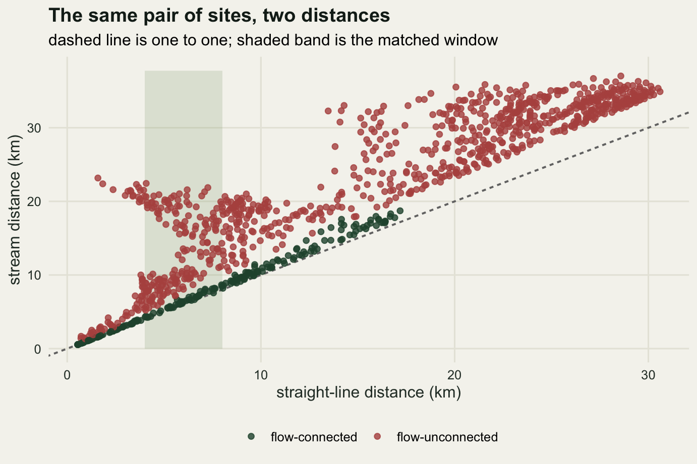
Substituting stream distance into a covariance function
The obvious move, having built a better distance, is to feed it to the machinery that already works. Take the exponential correlation function, replace the straight-line distance with the stream distance, and carry on. It is one character of code.
It is also not safe, and the reason is arithmetic rather than ecology. A covariance matrix has to be positive definite: every weighted average of the sites must have a non-negative variance under the model. A correlation function guarantees that only for the distances it was proved for, and the standard functions were proved for Euclidean distance in two or three dimensions. Curriero (2006) sets out the general version of the problem, and Ver Hoef (2018) works through what it does to network kriging. The three functions below are the three that the GLS post offers through corExp, corGaus and corSpher.
cf_exp <- function(h, a) exp(-h / a)
cf_gau <- function(h, a) exp(-(h / a)^2)
cf_sph <- function(h, a) ifelse(h < a, 1 - 1.5 * (h / a) + 0.5 * (h / a)^3, 0)
min_eig <- function(m) min(eigen(m, symmetric = TRUE, only.values = TRUE)$values)
The smallest test case is a star: several headwater tributaries meeting at one confluence, with a site some way up each. The stream distance between a site on tributary i and one on tributary j is the sum of their distances to the junction, so the whole matrix is fixed by the leg lengths.
star_dist <- function(leg) outer(leg, leg, "+") * (1 - diag(length(leg)))
leg7 <- 1:7
star7 <- star_dist(leg7)
rng_grid <- seq(2, 60, by = 0.01)
star_eig <- data.frame(
  rng = rng_grid,
  exponential = vapply(rng_grid, function(a) min_eig(cf_exp(star7, a)), numeric(1)),
  gaussian = vapply(rng_grid, function(a) min_eig(cf_gau(star7, a)), numeric(1)),
  spherical = vapply(rng_grid, function(a) min_eig(cf_sph(star7, a)), numeric(1)))

gau_fail <- star_eig$rng[which(star_eig$gaussian < 0)[1]]
gau_worst <- star_eig$rng[which.min(star_eig$gaussian)]
print(round(c(legs = length(leg7), max_stream_km = max(star7),
              gaussian_first_negative_km = gau_fail,
              gaussian_min_eigen = min(star_eig$gaussian),
              gaussian_worst_range_km = gau_worst,
              exponential_min_eigen = min(star_eig$exponential),
              spherical_min_eigen = min(star_eig$spherical)), 5))
legs max_stream_km
7.00000 13.00000
gaussian_first_negative_km gaussian_min_eigen
12.08000 -0.00813
gaussian_worst_range_km exponential_min_eigen
17.77000 0.04332
spherical_min_eigen
0.06471 Seven tributaries, one site 1 to 7 km up each. The exponential matrix stays positive definite across the whole sweep, with a smallest eigenvalue never below 0.0433. So does the spherical, never below 0.0647. The Gaussian does not: at a range of 12.08 km its smallest eigenvalue crosses zero, and by 17.77 km it is -0.00813.
A range of 12.08 km on a network whose longest stream distance is 13 km is not an unusual number to fit. Summer water temperature is correlated over tens of kilometres of channel, which is exactly the regime where this happens.
The real catchment is worse.
rng_grid2 <- seq(1, 100, by = 0.05)
catch_eig <- data.frame(
  rng = rng_grid2,
  exponential = vapply(rng_grid2, function(a) min_eig(cf_exp(str_d, a)), numeric(1)),
  gaussian = vapply(rng_grid2, function(a) min_eig(cf_gau(str_d, a)), numeric(1)),
  spherical = vapply(rng_grid2, function(a) min_eig(cf_sph(str_d, a)), numeric(1)))
print(round(c(gaussian_first_negative_km = catch_eig$rng[which(catch_eig$gaussian < 0)[1]],
              gaussian_negative_share = mean(catch_eig$gaussian < 0),
              gaussian_min_eigen = min(catch_eig$gaussian),
              exponential_min_eigen = min(catch_eig$exponential),
              spherical_min_eigen = min(catch_eig$spherical)), 5))
gaussian_first_negative_km gaussian_negative_share
2.05000 0.98940
gaussian_min_eigen exponential_min_eigen
-0.21797 0.00308
spherical_min_eigen
0.00461 On the forty-eight sites the Gaussian matrix has a negative eigenvalue at 98.9 per cent of the ranges swept, starting at 2.05 km, and reaching -0.218. The exponential and the spherical stay positive throughout.
A negative eigenvalue is not a numerical detail. Its eigenvector is a set of weights, and the model’s variance for that weighted average of the forty-eight temperatures is the eigenvalue itself.
a_bad <- 15
gau_bad <- cf_gau(str_d, a_bad)
ev <- eigen(gau_bad, symmetric = TRUE)
w_bad <- ev$vectors[, which.min(ev$values)]
var_bad <- as.numeric(t(w_bad) %*% gau_bad %*% w_bad)
chol_msg <- tryCatch({ chol(gau_bad); "succeeded" },
                     error = function(e) conditionMessage(e))
print(round(c(range_km = a_bad, model_variance_of_the_contrast = var_bad,
              sum_of_squared_weights = sum(w_bad^2),
              weights_above_point_two = sum(abs(w_bad) > 0.2),
              largest_weight = max(abs(w_bad))), 5))
range_km model_variance_of_the_contrast
15.00000 -0.09157
sum_of_squared_weights weights_above_point_two
1.00000 5.00000
largest_weight
0.68034 print(chol_msg)[1] "the leading minor of order 6 is not positive"At a range of 15 km there is a contrast, concentrated on 5 of the forty-eight sites, whose variance under the fitted model is -0.0916. No dataset can produce that. Everything downstream of the covariance matrix inherits the problem: chol() stops with the complaint that the leading minor of order 6 is not positive, so simulation from the model is impossible, and any routine that reaches the same matrix through a different factorisation will return kriging variances that can come out negative.
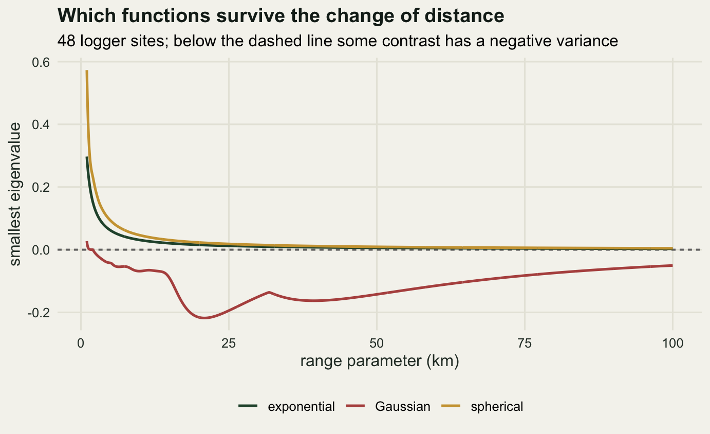
Two results out of one sweep is thin evidence, so the check below repeats it over three hundred randomly built catchments, each with a random number of levels, a random branching angle and a random set of sites, at twelve ranges each.
set.seed(20260801)
surv <- matrix(0, 0, 3)
for (rep_i in seq_len(300)) {
  nt <- build_network(n_level = sample(3:5, 1), len0 = runif(1, 5, 15),
                      shrink = runif(1, 0.5, 0.9), spread = runif(1, 0.3, 0.9),
                      n_piece = 3, seed = sample(1e6, 1))
  nn <- nrow(nt)
  sl <- sqrt((nt$x - nt$x[nt$parent])^2 + (nt$y - nt$y[nt$parent])^2)
  sl[is.na(sl)] <- 0
  od <- numeric(nn); dp <- vector("list", nn)
  for (i in seq_len(nn)) {
    p <- nt$parent[i]
    if (is.na(p)) { od[i] <- 0; dp[[i]] <- integer(0) }
    else { od[i] <- od[p] + sl[i]; dp[[i]] <- c(p, dp[[p]]) }
  }
  cjf <- function(i, j) { a <- c(i, dp[[i]]); b <- c(j, dp[[j]]); a[a %in% b][1] }
  st <- sort(sample(2:nn, min(nn - 1, sample(15:40, 1))))
  dm <- outer(od[st], od[st], "+") - 2 * od[outer(st, st, Vectorize(cjf))]
  for (a in exp(seq(log(0.5), log(500), length.out = 12)))
    surv <- rbind(surv, c(min_eig(cf_exp(dm, a)), min_eig(cf_gau(dm, a)),
                          min_eig(cf_sph(dm, a))))
}
colnames(surv) <- c("exponential", "gaussian", "spherical")
print(c(matrices = nrow(surv)))
matrices
3600 print(round(c(exp_fail = mean(surv[, 1] < 0), gau_fail = mean(surv[, 2] < 0),
sph_fail = mean(surv[, 3] < 0)), 4))exp_fail gau_fail sph_fail
0.0000 0.7494 0.0000 print(round(c(exp_worst = min(surv[, 1]), gau_worst = min(surv[, 2]),
sph_worst = min(surv[, 3])), 5))exp_worst gau_worst sph_worst
0.00019 -0.28191 0.00029 Over 3600 matrices the Gaussian fails 74.9 per cent of the time and gets as far as -0.2819. The exponential and the spherical never fail, and their worst smallest eigenvalues are 0.000192 and 0.000288, small but positive.
That result is not symmetrical, and the reason for the exponential is known: the distance along a tree can be laid out so that it becomes a sum of absolute differences, and the exponential function stays positive definite under distances of that kind. The spherical carries no such guarantee, and it is worth showing that it really is luck rather than law.
leg20 <- 1:20
star20 <- star_dist(leg20)
rng_grid3 <- seq(2, 200, by = 0.01)
sph20 <- vapply(rng_grid3, function(a) min_eig(cf_sph(star20, a)), numeric(1))
exp20 <- vapply(rng_grid3, function(a) min_eig(cf_exp(star20, a)), numeric(1))
print(round(c(branches = length(leg20),
              spherical_first_negative_km = rng_grid3[which(sph20 < 0)[1]],
              spherical_min_eigen = min(sph20),
              exponential_min_eigen = min(exp20)), 5))
branches spherical_first_negative_km
20.00000 26.49000
spherical_min_eigen exponential_min_eigen
-0.10669 0.01245 A junction with 20 tributaries entering it is not a real confluence, but it is a legal network, and on it the spherical function goes negative from a range of 26.49 km, down to -0.1067. The exponential still does not.
Now the sentence from the GLS post can be given its condition. On a plane, with Euclidean distance, all three functions are valid, the choice between exponential and spherical is a matter of fit, and refusing to agonise over it is the right call. The moment stream distance is substituted for Euclidean distance the choice stops being about fit: two of the three functions come through on ordinary dendritic networks, the Gaussian usually does not, and no amount of AIC will tell you which is which, because a model with a negative eigenvalue still returns a likelihood. On a network, pick the exponential, and pick it before looking at the data.
Building a tail-up covariance instead
Substituting a distance was the wrong move to begin with. The right one is to build the covariance from the process, and the construction that does it is a moving average over the network.
Put independent white noise everywhere on the channel. The value at a site is an integral of that noise over the part of the network upstream of the site, weighted by a kernel that decays with how far the noise has travelled down to the site. Nothing from a different tributary can enter, because nothing from a different tributary flows past. That is the tail-up model of Ver Hoef, Peterson and Theobald (2006) and Ver Hoef and Peterson (2010), and it delivers the two properties the substitution could not: covariance that is exactly zero between flow-unconnected sites, and positive definiteness by construction, because the covariance matrix is the cross-product of a design matrix and a cross-product cannot have a negative eigenvalue.
One detail makes it work at confluences. If the kernel simply carried on down past a junction, a site below a confluence would integrate over two tributaries’ worth of noise and have a larger variance than a site above it, which is not a model of anything. So the contribution from each incoming branch is multiplied by a weight, and the weights of the branches meeting at a junction sum to one. From the point of view of any site, the weighted network upstream of it then looks exactly like a single half-line, and every site has the same variance.
Two weighting rules are plausible. Split equally at every confluence, or split in proportion to what each branch delivers, for which upstream catchment area is the usual proxy. Areas are assigned to the headwaters here and accumulated downstream, which is what makes them additive.
set.seed(555)
tip_area <- exp(rnorm(length(head_tip), log(7), 0.5))
catch_area <- numeric(n_node)
for (i in rev(seq_len(n_node))) {
  catch_area[i] <- if (n_child[i] == 0) tip_area[match(i, head_tip)]
                   else sum(catch_area[which(net$parent == i)])
}
juncs <- which(n_child > 1)
sum_one <- vapply(juncs, function(j)
  sum(catch_area[which(net$parent == j)]) / catch_area[j], numeric(1))
area_ratio <- vapply(juncs, function(j) {
  ch <- which(net$parent == j)
  max(catch_area[ch]) / min(catch_area[ch])
}, numeric(1))
print(round(c(outlet_area_km2 = catch_area[1],
              headwater_area_min = min(tip_area), headwater_area_max = max(tip_area),
              confluence_weights_sum_to_one = max(abs(sum_one - 1)),
              confluence_ratio_median = median(area_ratio),
              confluence_ratio_max = max(area_ratio)), 5))
outlet_area_km2 headwater_area_min
123.77713 2.87473
headwater_area_max confluence_weights_sum_to_one
17.99727 0.00000
confluence_ratio_median confluence_ratio_max
1.47527 3.79152 The proportional influence of a branch is its share of the flow at the junction it enters. To get the weight between two flow-connected sites, multiply the proportional influences of every branch the water passes through on its way from the upper site to the lower one. The recursion below does that for every pair of nodes at once, going down the tree.
influence_matrix <- function(rule) {
  wt <- rep(1, n_node)
  for (v in 2:n_node) {
    p <- net$parent[v]
    if (n_child[p] > 1)
      wt[v] <- if (rule == "area") catch_area[v] / catch_area[p] else 1 / n_child[p]
  }
  pmat <- matrix(0, n_node, n_node)
  pmat[1, 1] <- 1
  for (v in 2:n_node) {
    pmat[v, ] <- pmat[net$parent[v], ] * wt[v]
    pmat[v, v] <- 1
  }
  pmat
}
pi_area <- influence_matrix("area")
pi_equal <- influence_matrix("equal")

telescope_gap <- max(vapply(2:n_node, function(v) {
  s <- down_path[[v]]
  max(abs(pi_area[v, s] - catch_area[v] / catch_area[s]))
}, numeric(1)))
print(signif(c(telescoping_check = telescope_gap), 3))
telescoping_check
5.55e-17 The check is worth pausing on. Under the area rule the product of proportional influences from one site down to another collapses to the ratio of their catchment areas, because every junction’s area is the sum of the areas entering it and the intermediate terms cancel. The two routes to the same number agree to 5.55e-17, which is floating point noise. The equal-split rule does not telescope: it is one half raised to the number of confluences passed, so it depends on how many junctions lie between two sites rather than on what those junctions carry.
The covariance follows. The variance of a site is the same everywhere by construction, the covariance between flow-unconnected sites is zero, and between flow-connected sites it is the square root of the accumulated influence times an exponential in stream distance. The square root is what keeps the variance constant: the moving average carries the square root of each branch weight, so squaring the kernel gives back the weights, and those add to one at every confluence. For a pair the accumulated influence enters once, from the lower site’s kernel.
weight_matrix <- function(pmat) {
  wm <- matrix(0, n_site, n_site)
  for (a in seq_len(n_site)) for (b in seq_len(n_site)) {
    if (a == b) { wm[a, b] <- 1; next }
    k <- junc[a, b]
    if (k == site_id[b]) wm[a, b] <- sqrt(pmat[site_id[a], site_id[b]])
    else if (k == site_id[a]) wm[a, b] <- sqrt(pmat[site_id[b], site_id[a]])
  }
  wm
}
w_area <- weight_matrix(pi_area)
w_equal <- weight_matrix(pi_equal)
tail_up <- function(a, wm) wm * exp(-str_d / a)

conn_off <- conn & !diag(n_site)
w_cor <- cor(w_area[conn_off], w_equal[conn_off])
print(round(c(symmetric = max(abs(w_area - t(w_area))),
              zeros_match_unconnected = sum((w_area > 0) != conn),
              area_weight_min = min(w_area[conn_off]),
              area_weight_median = median(w_area[conn_off]),
              equal_weight_min = min(w_equal[conn_off]),
              equal_weight_median = median(w_equal[conn_off]),
              weight_correlation = w_cor,
              sqrt_of_a_quarter = sqrt(0.25), sqrt_of_a_half = sqrt(0.5)), 4))
symmetric zeros_match_unconnected area_weight_min
0.0000 0.0000 0.1524
area_weight_median equal_weight_min equal_weight_median
0.4883 0.2500 0.5000
weight_correlation sqrt_of_a_quarter sqrt_of_a_half
0.9550 0.5000 0.7071 tu_eig <- vapply(c(1, 5, 10, 20, 50, 200),
function(a) min_eig(tail_up(a, w_area)), numeric(1))
print(round(setNames(tu_eig, paste0("range_", c(1, 5, 10, 20, 50, 200))), 5)) range_1 range_5 range_10 range_20 range_50 range_200
0.31792 0.06803 0.03421 0.01715 0.00687 0.00172 Every smallest eigenvalue is positive. That is not a lucky sweep, and the way to show it is to build the moving average explicitly and check that the analytic formula is what comes out. The network is cut into quadrature intervals; each headwater is extended upstream by eight ranges so the kernel is not truncated; and for every site a column is filled with the kernel value times the square root of the accumulated influence. The covariance is then the cross-product of that matrix, which is positive semi-definite whatever the numbers in it.
ma_cov <- function(a, pmat, delta = 0.02, n_rng = 8) {
  pieces <- list()
  for (v in 2:n_node) {
    if (seg_len[v] <= 0) next
    m <- ceiling(seg_len[v] / delta)
    pieces[[length(pieces) + 1]] <- list(
      base = out_dist[net$parent[v]], node = v, dl = seg_len[v] / m,
      u = (seq_len(m) - 0.5) * seg_len[v] / m, below = down_path[[v]])
  }
  for (tp in head_tip) {
    m <- ceiling(n_rng * a / delta)
    pieces[[length(pieces) + 1]] <- list(
      base = out_dist[tp], node = tp, dl = n_rng * a / m,
      u = (seq_len(m) - 0.5) * n_rng * a / m, below = c(tp, down_path[[tp]]))
  }
  sig <- matrix(0, n_site, n_site)
  for (pc in pieces) {
    idx <- match(pc$below, site_id)
    keep <- !is.na(idx)
    if (!any(keep)) next
    col_i <- idx[keep]
    nd <- pc$below[keep]
    dm <- outer(pc$u, pc$base - out_dist[nd], "+")
    gmat <- exp(-dm / a) * rep(sqrt(pmat[pc$node, nd]), each = length(pc$u)) *
      sqrt(pc$dl)
    sig[col_i, col_i] <- sig[col_i, col_i] + crossprod(gmat)
  }
  sig / (a / 2)
}
ma_tab <- t(vapply(c(3, 6, 12), function(a) {
  sm <- ma_cov(a, pi_area)
  c(range = a, max_gap = max(abs(sm - tail_up(a, w_area))),
    variance_gap = max(abs(diag(sm) - 1)), min_eigen = min_eig(sm))
}, numeric(4)))
print(signif(ma_tab, 4))
range max_gap variance_gap min_eigen
[1,] 3 7.520e-06 7.520e-06 0.11240
[2,] 6 1.964e-06 1.964e-06 0.05680
[3,] 12 5.755e-07 5.755e-07 0.02853The moving average and the analytic formula agree to 7.52e-06 at worst, which is quadrature error, and the constructed matrix has a smallest eigenvalue of 0.02853 at the longest range tested. The formula is not a guess that happens to work; it is the covariance of an explicit process, and that is where the positive definiteness comes from.
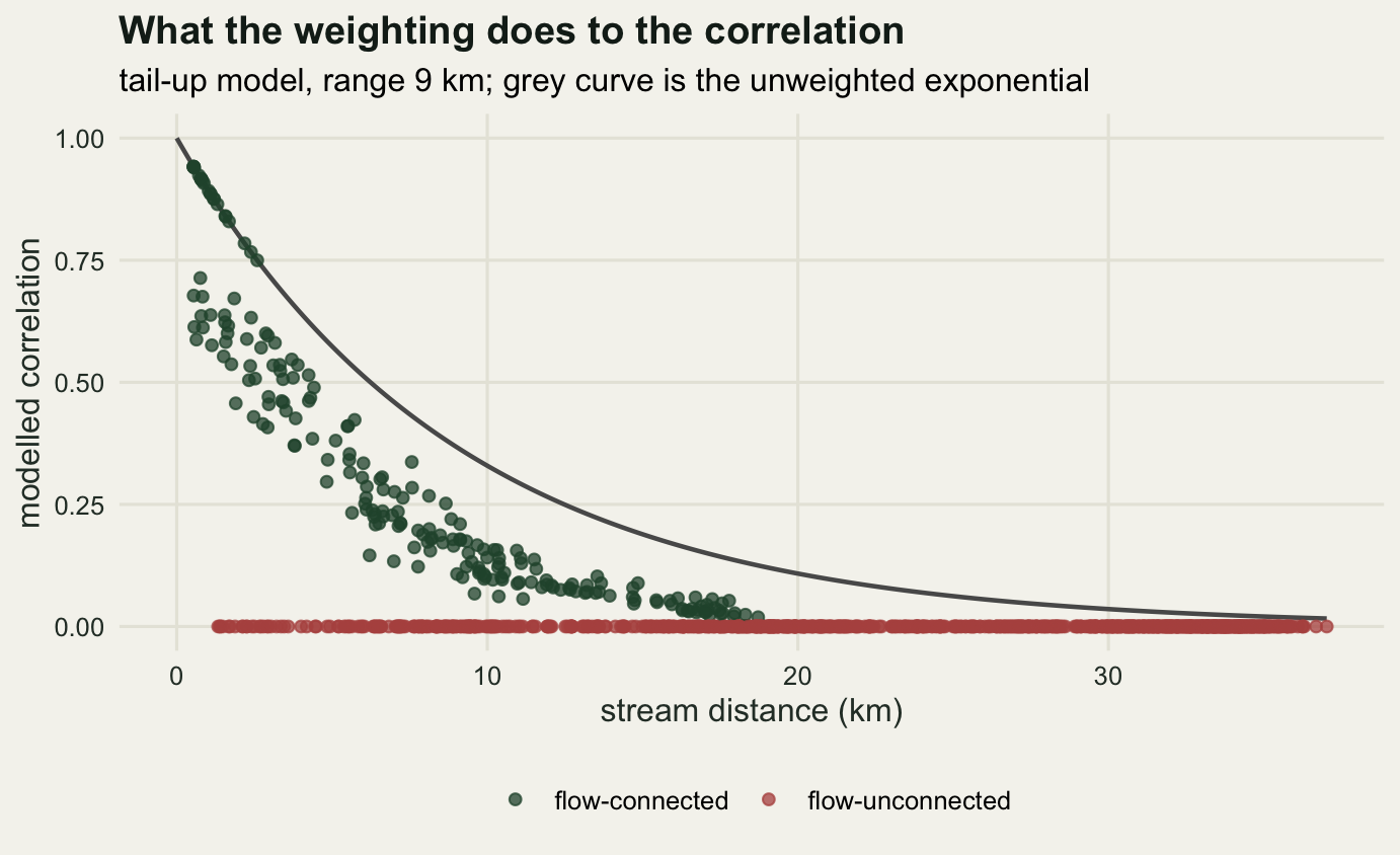
Fitting, and how much the weighting rule matters
The model is a constant mean plus a tail-up process plus a nugget, and it is fitted by restricted maximum likelihood: three parameters on the log scale, the mean profiled out by generalised least squares at every evaluation. The range gets an upper bound, and how often the optimiser reaches it turns out to matter.
rng_max <- 200
a_true <- 9
sill_true <- 1
nug_true <- 0.15
mu_true <- 14

neg2_reml <- function(vmat, y) {
  ch <- chol(vmat + diag(1e-10, nrow(vmat)))
  vinv <- chol2inv(ch)
  tot <- sum(vinv)
  mu <- sum(vinv %*% y) / tot
  err <- y - mu
  2 * sum(log(diag(ch))) + log(tot) + as.numeric(t(err) %*% vinv %*% err)
}

fit_reml <- function(y, covfun, start = c(0, log(6), -2)) {
  obj <- function(p) {
    if (p[2] < log(0.1) || p[2] > log(rng_max)) return(1e10)
    val <- tryCatch(neg2_reml(covfun(p) + diag(exp(p[3]), length(y)), y),
                    error = function(e) 1e10)
    if (is.finite(val)) val else 1e10
  }
  op <- optim(start, obj, method = "Nelder-Mead",
              control = list(maxit = 800, reltol = 1e-9))
  list(sill = exp(op$par[1]), rng = exp(op$par[2]), nug = exp(op$par[3]))
}

sim_tail_up <- function(a, sill, nug, mu, wm) {
  vmat <- sill * tail_up(a, wm) + diag(nug, n_site)
  mu + as.vector(t(chol(vmat)) %*% rnorm(n_site))
}
print(c(range_bound_km = rng_max, true_range_km = a_true,
        true_partial_sill = sill_true, true_nugget = nug_true,
        true_mean_degrees = mu_true))
range_bound_km true_range_km true_partial_sill true_nugget
200.00 9.00 1.00 0.15
true_mean_degrees
14.00 The bound on the range is 200 km, about five times the longest stream distance in the catchment. The truth used from here on is a tail-up process with area weighting, a range of 9 km, a partial sill of 1 and a nugget of 0.15 on a mean of 14 degrees, which puts the site standard deviation near one degree: a plausible summer temperature field for a catchment this size. The first question is what happens if the weighting rule is wrong, which is the part of a tail-up fit that a real analysis has least information about.
set.seed(7777)
n_wrep <- 200
wrep <- matrix(NA_real_, n_wrep, 2)
for (i in seq_len(n_wrep)) {
  y <- sim_tail_up(a_true, sill_true, nug_true, mu_true, w_area)
  wrep[i, ] <- c(
    fit_reml(y, function(p) exp(p[1]) * tail_up(exp(p[2]), w_area))$rng,
    fit_reml(y, function(p) exp(p[1]) * tail_up(exp(p[2]), w_equal))$rng)
}
colnames(wrep) <- c("correct_weights", "equal_split")
print(round(c(median_correct = median(wrep[, 1]), median_equal = median(wrep[, 2]),
              median_ratio = median(wrep[, 2] / wrep[, 1])), 4))
median_correct median_equal median_ratio
9.4785 9.7455 0.9912 print(round(c(q25_correct = unname(quantile(wrep[, 1], 0.25)),
q75_correct = unname(quantile(wrep[, 1], 0.75)),
at_upper_bound = sum(wrep[, 1] > rng_max - 1)), 3)) q25_correct q75_correct at_upper_bound
4.775 22.029 16.000 The rule barely moves the answer. With the correct weights the median fitted range over 200 replicates is 9.478 km against a truth of 9; with every confluence split equally it is 9.745 km, a median ratio of 0.9912. That difference is nothing beside the sampling spread of the range itself, whose quartiles across replicates run from 4.78 to 22.03 km, and in 16 of 200 replicates the correctly specified fit ran all the way to the upper bound.
The reason is in the weights, not in the fitting. The two rules correlate at 0.955 across the flow-connected pairs, because a tributary that carries a quarter of the flow and a tributary that carries a half give square roots of 0.5 and 0.707, and the square root flattens the disagreement. This catchment has confluences whose two branches differ in area by a factor of up to 3.79, and even so the two weightings are nearly the same matrix. If a real dataset cannot tell the two rules apart, that is because there is very little there to tell apart, which is a more useful thing to know than a rule of thumb about which proxy to use.
Prediction, measured
Now the question the loggers were put out to answer. Simulate a temperature field from the tail-up truth, hold out twelve of the forty-eight sites, fit to the remaining thirty-six and predict the held-out values three ways: with the tail-up model and the correct weights, with the tail-up model and equal splits, and with an exponential model on straight-line distance that knows nothing about the channel. The predictor is universal kriging with the mean estimated by generalised least squares, written out below.
krige_at <- function(sill, rng, nug, covfun, obs, hold, y_obs) {
  vinv <- chol2inv(chol(covfun(sill, rng, obs, obs) +
                          diag(nug + 1e-10, length(obs))))
  tot <- sum(vinv)
  mu <- sum(vinv %*% y_obs) / tot
  c0 <- covfun(sill, rng, obs, hold)
  wts <- vinv %*% c0
  lagr <- 1 - colSums(wts)
  list(pred = mu + as.vector(t(wts) %*% (y_obs - mu)),
       sd = sqrt(pmax(sill + nug - colSums(c0 * wts) + lagr^2 / tot, 1e-12)))
}
cov_area <- function(s, a, i, j) s * w_area[i, j, drop = FALSE] *
  exp(-str_d[i, j, drop = FALSE] / a)
cov_equal <- function(s, a, i, j) s * w_equal[i, j, drop = FALSE] *
  exp(-str_d[i, j, drop = FALSE] / a)
cov_euclid <- function(s, a, i, j) s * exp(-euc_d[i, j, drop = FALSE] / a)set.seed(1301)
n_rep <- 300
n_hold <- 12
nominal <- 0.95
z_crit <- qnorm(1 - (1 - nominal) / 2)
hold_res <- matrix(NA_real_, n_rep, 12)
for (i in seq_len(n_rep)) {
y <- sim_tail_up(a_true, sill_true, nug_true, mu_true, w_area)
hold <- sample(n_site, n_hold)
obs <- setdiff(seq_len(n_site), hold)
y_obs <- y[obs]
y_hold <- y[hold]
f1 <- fit_reml(y_obs, function(p)
exp(p[1]) * w_area[obs, obs] * exp(-str_d[obs, obs] / exp(p[2])))
f2 <- fit_reml(y_obs, function(p)
exp(p[1]) * w_equal[obs, obs] * exp(-str_d[obs, obs] / exp(p[2])))
f3 <- fit_reml(y_obs, function(p)
exp(p[1]) * exp(-euc_d[obs, obs] / exp(p[2])))
k1 <- krige_at(f1$sill, f1$rng, f1$nug, cov_area, obs, hold, y_obs)
k2 <- krige_at(f2$sill, f2$rng, f2$nug, cov_equal, obs, hold, y_obs)
k3 <- krige_at(f3$sill, f3$rng, f3$nug, cov_euclid, obs, hold, y_obs)
hold_res[i, ] <- c(
sqrt(mean((k1$pred - y_hold)^2)), sqrt(mean((k2$pred - y_hold)^2)),
sqrt(mean((k3$pred - y_hold)^2)),
mean(abs(k1$pred - y_hold) <= z_crit * k1$sd),
mean(abs(k2$pred - y_hold) <= z_crit * k2$sd),
mean(abs(k3$pred - y_hold) <= z_crit * k3$sd),
mean(k1$sd), mean(k2$sd), mean(k3$sd), f1$rng, f2$rng, f3$rng)
}
colnames(hold_res) <- c("rmse_tu", "rmse_eq", "rmse_euc", "cover_tu", "cover_eq",
"cover_euc", "sd_tu", "sd_eq", "sd_euc", "rng_tu",
"rng_eq", "rng_euc")
hold_res <- as.data.frame(hold_res)
print(round(colMeans(hold_res[, 1:9]), 4)) rmse_tu rmse_eq rmse_euc cover_tu cover_eq cover_euc sd_tu sd_eq
0.7273 0.7289 0.8504 0.9192 0.9178 0.9369 0.6926 0.6917
sd_euc
0.8481 print(round(c(rmse_ratio_euclid = mean(hold_res$rmse_euc / hold_res$rmse_tu),
rmse_ratio_equal = mean(hold_res$rmse_eq / hold_res$rmse_tu),
tailup_wins_pct = 100 * mean(hold_res$rmse_tu < hold_res$rmse_euc)), 4))rmse_ratio_euclid rmse_ratio_equal tailup_wins_pct
1.1983 1.0019 77.6667 The tail-up model predicts better. Over 300 replicates its hold-out root mean squared error is 0.7273 degrees against 0.8504 for the Euclidean model, a ratio of 1.1983 computed replicate by replicate, and it wins in 77.7 per cent of them. The equal-split version is indistinguishable from the correct one, 0.7289 against 0.7273, which is the previous section’s finding arriving again through a different door.
Interval coverage does not separate the models, and it does not go the way the accuracy does. Nominal ninety-five per cent intervals cover 91.9 per cent of held-out values under the tail-up model and 93.7 per cent under the Euclidean one, so the model that predicts worse has the marginally better calibrated intervals. The mechanism is in the next line of output: the Euclidean model’s average prediction standard deviation is 0.8481 against 0.6926, so it buys its coverage with intervals 22.4 per cent wider. Both models undercover, and the shortfall belongs to the plug-in step rather than to either geometry.
set.seed(99)
n_known <- 400
known_cov <- numeric(n_known)
for (i in seq_len(n_known)) {
  y <- sim_tail_up(a_true, sill_true, nug_true, mu_true, w_area)
  hold <- sample(n_site, n_hold)
  obs <- setdiff(seq_len(n_site), hold)
  k <- krige_at(sill_true, a_true, nug_true, cov_area, obs, hold, y[obs])
  known_cov[i] <- mean(abs(k$pred - y[hold]) <= z_crit * k$sd)
}
print(round(c(coverage_with_true_parameters = mean(known_cov)), 4))
coverage_with_true_parameters
0.9492 Feed the generating parameters to the same predictor and coverage returns to 94.9 per cent. The 3.1 point shortfall in the fitted case is the price of estimating three covariance parameters from thirty-six sites and then treating them as known, which is a general property of plug-in kriging rather than anything to do with networks.
The result with the largest practical reach is the last one, and it is about a number rather than about a map.
rng_tab <- data.frame(
  model = c("tail-up, correct weights", "tail-up, equal split",
            "Euclidean exponential"),
  median_range = c(median(hold_res$rng_tu), median(hold_res$rng_eq),
                   median(hold_res$rng_euc)),
  q25 = c(quantile(hold_res$rng_tu, 0.25), quantile(hold_res$rng_eq, 0.25),
          quantile(hold_res$rng_euc, 0.25)),
  q75 = c(quantile(hold_res$rng_tu, 0.75), quantile(hold_res$rng_eq, 0.75),
          quantile(hold_res$rng_euc, 0.75)),
  at_bound = c(sum(hold_res$rng_tu > rng_max - 1), sum(hold_res$rng_eq > rng_max - 1),
               sum(hold_res$rng_euc > rng_max - 1)))
print(rng_tab, row.names = FALSE, digits = 4)
model median_range q25 q75 at_bound
tail-up, correct weights 10.43 5.726 30.643 44
tail-up, equal split 10.81 5.833 27.879 43
Euclidean exponential 2.03 1.392 3.847 7print(round(c(true_range = a_true,
gap_factor = median(hold_res$rng_tu) / median(hold_res$rng_euc)), 4))true_range gap_factor
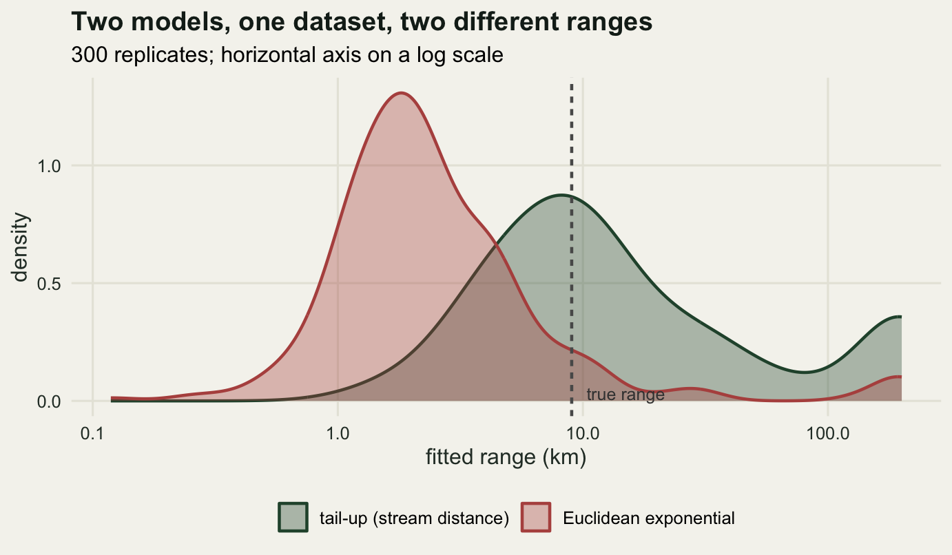
9.0000 5.1392 The tail-up range recovers the truth in the median, 10.431 km against 9, with quartiles from 5.73 to 30.64 and 44 replicates pinned at the bound. The Euclidean model fitted to the same data gives a median range of 2.03 km, 5.14 times smaller, with quartiles from 1.39 to 3.85.
Both numbers are called the range and both come out of a corExp structure, and a reader handed the second one will report that summer temperature is correlated over about 2 km. What the Euclidean model has actually done is average two incompatible things: it has to explain strong correlation between sites a few kilometres apart on one channel and near-zero correlation between sites the same distance apart across a divide, and the only way a single decaying function of straight-line distance can do both is to decay fast. The fitted parameter is a compromise between the two classes of pair, and the ecological reading of it, the length of channel over which conditions travel, is not what it measures. Getting 2 km instead of 10.4 km is not a small error in the same quantity. It is the right answer to a question about the plane.
What a pure tail-up model gets wrong
The model above says that two sites on different tributaries are independent. For a dissolved substance moving with the water, that is close to right, and it is the reason the tail-up predictor beat the Euclidean one. For most of what a freshwater ecologist measures it is wrong, and wrong in a direction that matters.
An adult stonefly flies. A grazing mammal walks between headwaters. Air temperature, geology, land use and rainfall do not respect the drainage divide either, and they drive a good share of the variation in a stream variable. Two sites on adjacent tributaries three hundred metres apart share almost all of their catchment context and none of their water, and a pure tail-up model gives them a covariance of exactly zero. That is the mirror image of the error the Euclidean model makes, and it is no more defensible. Peterson et al. (2013) argue the general version of this: a dendritic network is an ecological object with several kinds of connection running over it at once, not a single distance to be substituted into an existing model.
The standard answer is a mixture. A tail-down component allows correlation between flow-unconnected sites through their shared downstream junction, which covers things that move upstream as well as down. A Euclidean component covers everything that arrives from the air or from the land surface. The covariance is a sum of the three, each with its own partial sill and range, and Peterson and Ver Hoef (2010) set the mixture out in the form that the software implements.
The honest problem with the mixture is that its weights are hard to identify. Fitting it means estimating at least six covariance parameters, and the previous section could not pin down one range from thirty-six sites: the quartiles ran from 5.73 to 30.64 km and 44 of 300 fits hit the upper bound with the model correctly specified and the weighting rule known. A typical stream network study has thirty to sixty sites. Isaak et al. (2014) review what the models have been applied to, and the applications that resolve a mixture cleanly tend to be the ones with hundreds of sites and several years of data. With fifty sites the sensible report is the fitted mixture proportions with a plain statement that the data cannot separate the components, not a story about which process dominates.
Three smaller limits are worth naming. The weights here came from a synthetic catchment area that was built to be additive; on a real network the additive function has to be computed from a digital elevation model and a stream layer, and getting it topologically correct is most of the work. The nugget in this simulation is a real nugget, but on a stream network some of what looks like a nugget is variation at a scale finer than the segment resolution of the layer, so it moves when the layer changes. And every number here comes from one synthetic catchment shape: the positive-definiteness survey covered three hundred network shapes, but the prediction and weighting results did not.
For a real catchment the calculations above are done by dedicated software rather than by hand. The block below does not run.
# SSN2::ssn_import("catchment.ssn", predpts = "preds")
# SSN2::ssn_lm(temp ~ elev, ssn.object = net_ssn,
#              tailup_type = "exponential", taildown_type = "exponential",
#              euclid_type = "exponential", additive = "afvArea")
# openSTARS::derive_streams()   # builds the .ssn from a DEM in GRASS
SSN2 (Dumelle et al. 2024) is the current implementation and replaces the older SSN package; openSTARS builds the network object from a digital elevation model. Cressie et al. (2006) is the other early treatment of prediction on a river network and reaches the flow-connected covariance from a different direction.
What to take away
Stream distance and straight-line distance agree closely along a single channel: over the forty-eight sites here the flow-connected pairs correlate at 0.9972 between the two measures, with a stream-to-straight ratio never above 1.24. Between sites on different tributaries they do not: 0.9133, and one pair 1.58 km apart on the map is 23.17 km apart along the water. The split into flow-connected and flow-unconnected pairs is the part with no counterpart on a plane, and it is what makes a network model a different object rather than a corrected distance.
Substituting stream distance into a standard correlation function is not a free move. On the forty-eight sites the Gaussian function produced a negative eigenvalue at 98.9 per cent of the ranges swept, and over 3600 matrices from three hundred random catchments it failed 74.9 per cent of the time. The exponential never failed. The spherical never failed on a dendritic network either but did fail on a twenty-branch star, so its survival is a property of the shapes real catchments take rather than a guarantee. The advice in the GLS post not to agonise between decay shapes holds on a plane and stops holding here, and the failure is silent: a likelihood still comes back, an AIC still gets computed, and only chol() complains.
Building the covariance from the moving average instead gives a matrix that is positive definite because it is a cross-product, and the explicit construction matched the analytic formula to 7.52e-06. Two results from that model went against what I expected. The weighting rule at confluences, which is the piece of a tail-up specification that gets the most attention, moved the median fitted range only from 9.48 km to 9.75 km when replaced by a crude equal split, and made no difference at all to hold-out error (0.7273 against 0.7289); the square root in the weight flattens the disagreement between the rules. And interval coverage did not follow accuracy: the Euclidean model predicted 16.9 per cent worse by root mean squared error and still covered slightly better, 93.7 against 91.9 per cent, because its intervals were 22.4 per cent wider. If the comparison in this post had been run on coverage alone it would have found nothing.
The number to be most careful with is the range. Fitted on stream distance it came out at 10.43 km against a truth of 9; fitted on straight-line distance to the same data it came out at 2.03 km. Both appear in output as a range in kilometres, and the smaller one is not a biased estimate of the larger. It is a summary of a different geometry, and reporting it as the length of channel over which conditions persist is the mistake this post exists to prevent.
References
Ver Hoef JM, Peterson EE 2010 Journal of the American Statistical Association 105(489):6-18 (10.1198/jasa.2009.ap08248)
Ver Hoef JM, Peterson EE, Theobald D 2006 Environmental and Ecological Statistics 13(4):449-464 (10.1007/s10651-006-0022-8)
Peterson EE, Ver Hoef JM 2010 Ecology 91(3):644-651 (10.1890/08-1668.1)
Cressie N, Frey J, Harch B, Smith M 2006 Journal of Agricultural, Biological, and Environmental Statistics 11(2):127-150 (10.1198/108571106X110649)
Curriero FC 2006 Mathematical Geology 38(8):907-926 (10.1007/s11004-006-9055-7)
Ver Hoef JM 2018 Methods in Ecology and Evolution 9(6):1600-1613 (10.1111/2041-210X.12979)
Peterson EE, et al 2013 Ecology Letters 16(5):707-719 (10.1111/ele.12084)
Isaak DJ, et al 2014 WIREs Water 1(3):277-294 (10.1002/wat2.1023)
Dumelle M, Peterson EE, Ver Hoef JM, Pearse A, Isaak DJ 2024 Journal of Open Source Software 9(99):6389 (10.21105/joss.06389)