library(ggplot2)
library(patchwork)

te_paper  <- "#f5f4ee"
te_ink    <- "#16241d"
te_body   <- "#2c3a31"
te_forest <- "#275139"
te_rust   <- "#b5534e"
te_gold   <- "#c9b458"
te_line   <- "#dad9ca"

theme_datasheet <- function() {
  theme_minimal(base_size = 12) +
    theme(plot.background  = element_rect(fill = te_paper, colour = NA),
          panel.background = element_rect(fill = te_paper, colour = NA),
          panel.grid.major = element_line(colour = te_line, linewidth = 0.3),
          panel.grid.minor = element_blank(),
          text             = element_text(colour = te_body),
          plot.title       = element_text(colour = te_ink, face = "bold"),
          plot.subtitle    = element_text(colour = te_body),
          axis.text        = element_text(colour = te_body))
}Spatial capture-recapture on a meandering stream
R
capture-recapture
spatial
abundance
freshwater
ecology tutorial
A planar SCR model on a meandering stream inflates abundance and shrinks sigma. Measuring in R which error a habitat mask fixes and which needs stream distance.
A crew is estimating the number of adult crayfish in a lowland reach. Baited traps sit in the channel every 250 m, the reach is walked on five occasions, and every animal is marked. The reach itself is nine kilometres of water inside five kilometres of valley: it swings back on itself so tightly that two traps a few hundred metres apart on the map can be more than a kilometre apart along the water.
The analyst opens an SCR script, buffers the reach by four times the expected sigma, lays a mask over the result and fits a half-normal detection function on straight-line distance. The state space is now mostly hay meadow and woodland, which no crayfish has ever occupied, and the distance from a trap on one limb of a bend to a trap on the next is measured across the neck rather than around it. Both of those are wrong, and they are wrong in different ways: one is a statement about where animals can be, the other a statement about how far apart two points are.
Spatial capture-recapture from scratch builds exactly that planar model: a rectangular grid of activity centres, Euclidean distances, a buffered box, and a takeaway that SCR “estimates density directly with a principled effective sampling area”. The principle holds; the effective sampling area is estimated rather than chosen. What the stream case breaks is the assumption underneath it, that the state space is the region the animal could occupy. SCR sampling design and precision then shows how trap spacing relative to sigma governs whether sigma can be pinned down at all, on a plane. This post keeps the same likelihood and changes the geometry.
Stream networks and tail-up covariance already put two distances side by side on a river, but for a covariance function between fixed sites, not for a detection function or for a set of places an animal can live. Its section on the two distances notes that along one thread of water, stream distance is straight-line distance multiplied by the sinuosity of the channel. That multiplier is the whole of the problem here, and it enters the SCR likelihood twice: once through the detection function and once through the state space. The same geometry damages a planar home range: a kernel density surface fitted to positions along a meandering stream, as in home ranges in R: MCP versus kernel density, spreads probability across the meander necks, so the 95 per cent contour contains land the animal never used.
The result that a linear state space and a network distance repair a stream SCR analysis is not new. Royle et al. 2013 introduced SCR with an ecological distance, and Sutherland, Fuller and Royle 2015 applied a network version to stream salamanders. The state space as a habitat mask goes back to Efford 2004 and Borchers and Efford 2008. The Sutherland et al. simulation was run on a riparian habitat network, and its headline is not the one this post reaches, which is worth saying here rather than at the end. They report that the ecological-distance model always produced unbiased estimates of abundance, while the Euclidean fit became negatively biased for abundance as space use tightened onto the water and gave a poor description of home range shape and no information about connectivity; Royle et al. 2013 likewise report that ignoring landscape connectivity biases density downwards. The masked Euclidean fit measured below is not biased downwards. Two things differ. Their state space is a two-dimensional landscape with a resistance surface, so parts of the mask are hard for an animal to reach and a Euclidean fit still credits animals to them; here the truth is strictly one-dimensional and the mask is the habitat itself, so that source of error has been removed by construction. And the repair measured here is conditional: the last section widens the trap spacing until the masked Euclidean fit fails. What this post measures is the split between the two errors, made explicit: which of them each repair removes, how the damage moves with sinuosity, and where the cheaper repair stops working.
A reach that is longer than the valley it crosses
The planform is a sine-generated curve, the shape Leopold and Langbein 1966 argued a meandering river takes: the channel direction, not the channel position, varies as a sine wave of distance along the channel. Writing the direction at arc length s as omega * cos(2 * pi * s / lambda), the sinuosity of a whole number of wavelengths is 1 / J0(omega), where J0 is the Bessel function of the first kind and order zero. That gives an exact handle on sinuosity and a curve with rounded bends rather than the cusps a sine drawn in valley coordinates produces at high amplitude.
lambda_m   <- 1.5      # meander wavelength along the channel, km
sigma_true <- 0.5      # true movement scale, km
p0_true    <- 0.15     # per-occasion detection at zero distance
n_occ      <- 5        # trapping occasions
dens_km    <- 8        # activity centres per km of channel
arc_trap   <- 9.0      # trapped length of channel, km
arc_buf    <- 1.5      # channel buffer each end, km (3 sigma)
arc_total  <- arc_trap + 2 * arc_buf
buf_planar <- 2.0      # planar mask buffer, km (4 sigma)
rip_half   <- 0.2      # riparian mask half width, km
cell_plan  <- 0.2      # planar mask cell side, km
cell_rip   <- 0.1      # riparian mask cell side, km
cell_line  <- 0.025    # channel line cell length, km

make_channel <- function(omega, ds = 0.002) {
  s_arc <- seq(0, arc_total, by = ds)
  ang   <- omega * cos(2 * pi * s_arc / lambda_m)
  x_pos <- c(0, cumsum((cos(ang[-1]) + cos(ang[-length(ang)])) / 2 * ds))
  y_pos <- c(0, cumsum((sin(ang[-1]) + sin(ang[-length(ang)])) / 2 * ds))
  list(s = s_arc, x = x_pos, y = y_pos)
}
omega_for <- function(target) {
  uniroot(function(w) 1 / besselJ(w, 0) - target, c(0.01, 2.2))$root
}

sinu_set  <- c(1.10, 1.45, 1.85, 2.70)
omega_set <- vapply(sinu_set, omega_for, 0)
sinu_draw <- vapply(omega_set, function(w) {
  ch <- make_channel(w)
  arc_total / sqrt(diff(range(ch$x[c(1, length(ch$x))]))^2 +
                   diff(range(ch$y[c(1, length(ch$y))]))^2)
}, 0)
sinu_gap  <- max(abs(sinu_draw - sinu_set))
bend_rad  <- lambda_m / (2 * pi * omega_set)
Four sinuosities are used throughout, 1.10, 1.45, 1.85 and 2.70. They are fixed before any simulation runs. The Bessel identity is worth checking rather than trusting: measuring the drawn curves gives sinuosities that differ from the targets by at most 0.000019, which is the numerical error of the integration and nothing else. The tightest bend radius runs from 391 m at the straightest setting down to 137 m at the most sinuous.
The channel length is held fixed at 12 km, with traps over the middle 9 km. Holding the channel fixed rather than the valley keeps the population, the number of traps and the trapping effort constant, so sinuosity is the only thing that moves. Because detection depends only on along-stream distance and the traps sit at the same arc positions in every design, the capture histories are drawn from one and the same distribution at all four sinuosities: nothing but the fitted geometry changes. Under the opposite convention, valley length held fixed and the channel growing with sinuosity, the planar mask would grow instead of shrinking, so the direction the mask area moves is a property of the convention. Activity centres are drawn uniformly along the channel at 8 per km, detection is half-normal on along-stream distance with sigma 0.50 km and p0 0.15, and each animal is exposed to every trap on 5 occasions.
Three state spaces are built over the same channel. The planar mask holds every cell within 2.0 km of the channel, which is four times the true sigma and is what a default buffer produces. The riparian mask holds every cell within 200 m of the channel. The channel line is the channel itself, cut into 25 m segments.
build_design <- function(omega, trap_gap = 0.25, rip_cell = cell_rip) {
  ch <- make_channel(omega)
  at_arc <- function(a) cbind(approx(ch$s, ch$x, a)$y, approx(ch$s, ch$y, a)$y)
  trap_s  <- seq(arc_buf, arc_buf + arc_trap, by = trap_gap)
  trap_xy <- at_arc(trap_s)

  idx <- seq(1, length(ch$s), by = 5)
  cx  <- ch$x[idx]; cy <- ch$y[idx]; cs <- ch$s[idx]
  nearest <- function(pts) {
    out_s <- numeric(nrow(pts)); out_d <- numeric(nrow(pts))
    blocks <- split(seq_len(nrow(pts)), ceiling(seq_len(nrow(pts)) / 400))
    for (b in blocks) {
      d2 <- outer(pts[b, 1], cx, "-")^2 + outer(pts[b, 2], cy, "-")^2
      w  <- max.col(-d2, "first")
      out_s[b] <- cs[w]; out_d[b] <- sqrt(d2[cbind(seq_along(b), w)])
    }
    list(s = out_s, d = out_d)
  }
  grid_of <- function(pad, step) {
    as.matrix(expand.grid(x = seq(min(ch$x) - pad, max(ch$x) + pad, by = step),
                          y = seq(min(ch$y) - pad, max(ch$y) + pad, by = step)))
  }
  gp  <- grid_of(buf_planar, cell_plan)
  np  <- nearest(gp)
  box_cells <- gp[np$d <= buf_planar, , drop = FALSE]
  gr  <- grid_of(2 * rip_half, rip_cell)
  nr  <- nearest(gr)
  keep_r <- nr$d <= rip_half
  rip <- gr[keep_r, , drop = FALSE]

  line_s <- seq(cell_line / 2, arc_total - cell_line / 2, by = cell_line)
  list(ch = ch, trap_s = trap_s, trap_xy = trap_xy,
       box = box_cells, w_box = rep(cell_plan^2, nrow(box_cells)),
       d_box = sqrt(outer(box_cells[, 1], trap_xy[, 1], "-")^2 +
                    outer(box_cells[, 2], trap_xy[, 2], "-")^2),
       rip = rip, w_rip = rep(rip_cell^2, nrow(rip)),
       d_rip_e = sqrt(outer(rip[, 1], trap_xy[, 1], "-")^2 +
                      outer(rip[, 2], trap_xy[, 2], "-")^2),
       d_rip_n = abs(outer(nr$s[keep_r], trap_s, "-")),
       line_s = line_s, w_line = rep(cell_line, length(line_s)),
       d_line = abs(outer(line_s, trap_s, "-")),
       d_line_e = sqrt(outer(at_arc(line_s)[, 1], trap_xy[, 1], "-")^2 +
                       outer(at_arc(line_s)[, 2], trap_xy[, 2], "-")^2))
}

des <- lapply(omega_set, build_design)
area_box <- vapply(des, function(d) sum(d$w_box), 0)
area_rip <- vapply(des, function(d) sum(d$w_rip), 0)
area_trp <- vapply(des, function(d)
  sum(d$w_box[apply(d$d_box, 1, min) <= buf_planar]), 0)
n_traps  <- length(des[[1]]$trap_s)
With the channel length fixed, a more sinuous reach coils into a smaller footprint, so the planar mask shrinks: 58.1 km2 at sinuosity 1.10 against 33.2 km2 at 2.70. The riparian mask does not follow it down: it is constant to better than one per cent at the first three settings, 4.86, 4.86 and 4.89 km2, and then drops to 3.99 km2 at the tightest. A strip of constant half width wrapped around a curve of fixed length has an area of about 4.80 km2 however the curve is bent, and it only loses area where the strip runs into itself, which happens here at the tightest bends and not before. Every design carries 37 traps.
One convention inside the planar mask is worth stating, because the estimated abundance is directly proportional to the state space. The buffer is taken around the whole 12 km of channel, including the 1.5 km of untrapped water at each end, and not around the trap array: that is what a mask built from a mapped reach gives. Buffering the 37 traps instead would give 46.9 km2 at the straightest setting and 28.4 km2 at the most sinuous, between 1.17 and 1.24 times smaller, and because those extra cells lie more than 2.0 km from every trap and add almost nothing to the effectively searched area, a reader whose software buffers the traps should expect a planar inflation smaller by roughly that same factor.
shift_y <- c(2.75, -2.75)
map_dat <- function(k, tag) {
  d <- des[[k]]; dy <- shift_y[tag]
  list(box  = data.frame(x = d$box[, 1], y = d$box[, 2] + dy),
       rip  = data.frame(x = d$rip[, 1], y = d$rip[, 2] + dy),
       chan = data.frame(x = d$ch$x, y = d$ch$y + dy),
       trap = data.frame(x = d$trap_xy[, 1], y = d$trap_xy[, 2] + dy),
       lab  = data.frame(x = -1.9, y = dy + 2.15,
                         t = sprintf("sinuosity %.2f, planar mask %.1f km2, riparian mask %.2f km2",
                                     sinu_set[k], area_box[k], area_rip[k])))
}
m_a <- map_dat(1, 1); m_b <- map_dat(4, 2)
ggplot() +
  geom_point(data = rbind(m_a$box, m_b$box), aes(x, y), colour = te_line, size = 0.3) +
  geom_point(data = rbind(m_a$rip, m_b$rip), aes(x, y), colour = te_gold, size = 0.3) +
  geom_path(data = m_a$chan, aes(x, y), colour = te_forest, linewidth = 0.45) +
  geom_path(data = m_b$chan, aes(x, y), colour = te_forest, linewidth = 0.45) +
  geom_point(data = rbind(m_a$trap, m_b$trap), aes(x, y), colour = te_rust, size = 0.8) +
  geom_text(data = rbind(m_a$lab, m_b$lab), aes(x, y, label = t),
            hjust = 0, size = 3.3, colour = te_body) +
  coord_equal(ylim = c(-5.3, 5.6)) +
  labs(x = "km", y = "km", title = "Same channel, three state spaces",
       subtitle = "grey: planar mask; gold: riparian mask; dark line: the channel; red points: traps") +
  theme_datasheet()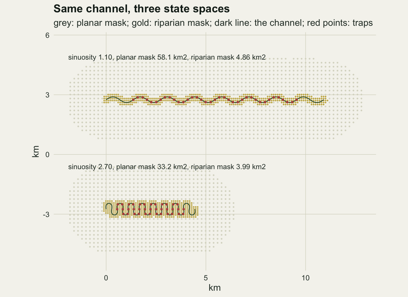
One likelihood, two state spaces, two distances
The likelihood is the Borchers and Efford 2008 form used in the earlier SCR post, written once and handed a distance matrix and a set of cell weights. Activity centres follow a Poisson process of intensity D over the state space; an animal with a centre in cell g is caught at trap j on a binomial number of the 5 occasions with per-occasion probability p0 * exp(-d(g, j)^2 / (2 * sigma^2)). Cell weights are areas in km2 for the two planar masks and lengths in km for the channel line, so D is per km2 in one case and per km in the other, and abundance in the state space is D times the total weight either way.
neg_ll <- function(par, caps, dmat, cellw) {
  p0 <- plogis(par[1]); sg <- exp(par[2]); dens <- exp(par[3])
  p_mat <- p0 * exp(-dmat^2 / (2 * sg^2))
  l_hit <- log(pmax(p_mat, 1e-300))
  l_mis <- log1p(-pmin(p_mat, 1 - 1e-12))
  l_cap <- caps %*% t(l_hit) + (n_occ - caps) %*% t(l_mis)
  p_dot <- 1 - exp(rowSums(n_occ * l_mis))
  mx    <- apply(l_cap, 1, max)
  l_marg <- mx + log(as.vector(exp(l_cap - mx) %*% cellw))
  -(sum(l_marg) + nrow(caps) * log(dens) - dens * sum(p_dot * cellw))
}

fit_scr <- function(caps, dmat, cellw, dens_start) {
  par_start <- c(qlogis(0.12), log(0.4), log(dens_start))
  op <- optim(par_start, neg_ll, caps = caps, dmat = dmat, cellw = cellw,
              method = "BFGS", control = list(maxit = 300, reltol = 1e-10))
  sg  <- exp(op$par[2])
  pd  <- 1 - exp(rowSums(n_occ * log1p(-pmin(plogis(op$par[1]) *
           exp(-dmat^2 / (2 * sg^2)), 1 - 1e-12))))
  c(abundance = exp(op$par[3]) * sum(cellw), sigma = sg, p0 = plogis(op$par[1]),
    area_eff = sum(pd * cellw), area_ss = sum(cellw), code = op$convergence)
}

simulate_survey <- function(d) {
  n_true <- rpois(1, dens_km * arc_total)
  cen_s  <- runif(n_true, 0, arc_total)
  p_mat  <- p0_true * exp(-outer(cen_s, d$trap_s, "-")^2 / (2 * sigma_true^2))
  caps   <- matrix(rbinom(length(p_mat), n_occ, p_mat), n_true)
  list(n_true = n_true, caps = caps[rowSums(caps) > 0, , drop = FALSE])
}
One survey at sinuosity 1.85 makes the pattern visible before any replication. Four models are fitted to the same capture histories, and a fifth, the channel line with straight-line distance, is added here alone to separate the distance from the state space at zero mask width.
set.seed(20260922)
d3  <- des[[3]]
one <- simulate_survey(d3)
caps_one <- one$caps
n_det    <- nrow(caps_one)
n_recap  <- sum(rowSums(caps_one > 0) > 1)

fit_one <- rbind(
  planar_euc   = fit_scr(caps_one, d3$d_box,    d3$w_box,  one$n_true / area_box[3]),
  riparian_euc = fit_scr(caps_one, d3$d_rip_e,  d3$w_rip,  one$n_true / area_rip[3]),
  riparian_net = fit_scr(caps_one, d3$d_rip_n,  d3$w_rip,  one$n_true / area_rip[3]),
  line_net     = fit_scr(caps_one, d3$d_line,   d3$w_line, dens_km),
  line_euc     = fit_scr(caps_one, d3$d_line_e, d3$w_line, dens_km))

id_check <- max(abs(fit_one[, "abundance"] -
                    n_det * fit_one[, "area_ss"] / fit_one[, "area_eff"]))
The survey caught 66 of 77 animals, and 55 of them were caught at more than one trap. On the channel line with along-stream distance the fit returns an abundance of 80 and a sigma of 0.529 km. On the planar mask with straight-line distance the same data give 350 animals and a sigma of 0.313 km. The riparian mask with straight-line distance gives 81 and 0.311; switching that model to along-stream distance moves the sigma to 0.529 and barely touches the abundance, at 81. The channel line with straight-line distance, which has no spare land at all, still returns a sigma of 0.312 km, and an abundance of 79, within one animal of the along-stream fit on the same state space. The shrinkage belongs to the distance and not to the width of the mask; the count belongs to the state space and not to the metric.
There is an identity behind the abundance figures that is worth writing down, because it lets the inflation be split into two measurable pieces. Profiling the likelihood over D gives D = n / a_eff, where a_eff is the integral of the detection probability over the state space, so the estimated abundance is exactly the number detected times the state space divided by the effectively searched area:
\[\hat N \;=\; n \, \frac{|S|}{a_{\text{eff}}}\]
This is a re-description of the estimator rather than a claim about the data: it holds for every fit by construction, and computing both sides for the five fits above agrees to 0.0006 of an animal, which is the optimiser’s convergence tolerance and tests nothing. What it buys is the split. The planar mask does not inflate the count because it has more area in some abstract sense; it inflates the count because most of that area is land where a crayfish would rarely be caught, so a_eff falls away from |S| and the ratio grows. Whether the gap between them widens with sinuosity is then a question about a_eff, and a_eff depends on the fitted sigma as well as on the mask.
The count follows the state space, the range and the growth follow the distance
The four fits are now run over the four sinuosities, on fresh capture histories each time. Trap spacing is 250 m throughout this section, which is half of the true sigma.
n_rep_main <- 14
run_cell <- function(d, n_rep, with_box = TRUE) {
  out <- replicate(n_rep, {
    sv <- simulate_survey(d)
    fa <- if (with_box) fit_scr(sv$caps, d$d_box, d$w_box, sv$n_true / sum(d$w_box)) else
      c(abundance = NA, sigma = NA, p0 = NA, area_eff = NA, area_ss = NA, code = 0)
    fb <- fit_scr(sv$caps, d$d_rip_e, d$w_rip,  sv$n_true / sum(d$w_rip))
    fc <- fit_scr(sv$caps, d$d_rip_n, d$w_rip,  sv$n_true / sum(d$w_rip))
    fd <- fit_scr(sv$caps, d$d_line,  d$w_line, dens_km)
    unname(c(sv$n_true, nrow(sv$caps),
             fa["abundance"], fa["sigma"], fa["area_eff"],
             fb["abundance"], fb["sigma"], fb["area_eff"],
             fc["abundance"], fc["sigma"], fd["abundance"], fd["sigma"],
             fa["code"] + fb["code"] + fc["code"] + fd["code"]))
  })
  out <- as.data.frame(t(out))
  names(out) <- c("n_true", "n_det", "N_box", "s_box", "aeff_box",
                  "N_rip", "s_rip", "aeff_rip", "N_ripn", "s_ripn",
                  "N_line", "s_line", "code")
  out
}
set.seed(51207)
grid_raw <- lapply(des, run_cell, n_rep = n_rep_main)
code_bad <- sum(vapply(grid_raw, function(g) sum(g$code), 0))

summar <- function(g, k) {
  rat <- function(v) c(mean(v), sd(v) / sqrt(nrow(g)))
  data.frame(
    sinuosity = sinu_set[k],
    model = c("planar mask, straight line", "riparian mask, straight line",
              "riparian mask, along stream", "channel line, along stream"),
    n_ratio = c(rat(g$N_box / g$n_true)[1], rat(g$N_rip / g$n_true)[1],
                rat(g$N_ripn / g$n_true)[1], rat(g$N_line / g$n_true)[1]),
    n_se    = c(rat(g$N_box / g$n_true)[2], rat(g$N_rip / g$n_true)[2],
                rat(g$N_ripn / g$n_true)[2], rat(g$N_line / g$n_true)[2]),
    sigma   = c(mean(g$s_box), mean(g$s_rip), mean(g$s_ripn), mean(g$s_line)),
    sigma_se = c(sd(g$s_box), sd(g$s_rip), sd(g$s_ripn), sd(g$s_line)) / sqrt(nrow(g)))
}
grid_tab <- do.call(rbind, lapply(seq_along(des), function(k) summar(grid_raw[[k]], k)))
grid_tab$model <- factor(grid_tab$model, levels = unique(grid_tab$model))
det_frac <- mean(unlist(lapply(grid_raw, function(g) g$n_det / g$n_true)))
pick <- function(m, k, col) grid_tab[[col]][grid_tab$model == levels(grid_tab$model)[m] &
                                            grid_tab$sinuosity == sinu_set[k]]
All 224 fits converged, with 0 non-zero optimiser codes, and on average 0.84 of the animals present were caught at least once.
The planar mask with straight-line distance returns 2.75 times the true abundance at sinuosity 1.10 and 6.19 times at sinuosity 2.70, with Monte Carlo standard errors of 0.049 and 0.108. The error grows with sinuosity even though the mask itself is getting smaller, which rules out the reading that the inflation is simply the area the box adds. Clipping the state space to the riparian strip removes almost all of it: 1.05 and 1.06 at the same two sinuosities, with the straight-line distance still in place. The correctly specified model on the channel line sits at 1.02 and 1.02, so a few per cent of the riparian mask’s residual is the small-sample behaviour of the estimator rather than anything geometric.
p_all <- ggplot(grid_tab, aes(sinuosity, n_ratio, colour = model)) +
  geom_hline(yintercept = 1, linetype = "dashed", colour = te_body, linewidth = 0.5) +
  geom_errorbar(aes(ymin = n_ratio - 1.96 * n_se, ymax = n_ratio + 1.96 * n_se),
                width = 0.04, linewidth = 0.4) +
  geom_line(linewidth = 0.9) +
  geom_point(size = 2.2) +
  scale_y_log10(breaks = c(1, 1.5, 2, 3, 5, 7)) +
  scale_colour_manual(values = c(te_rust, te_gold, te_forest, te_ink),
                      name = NULL, drop = FALSE) +
  labs(x = "channel sinuosity", y = "estimated / true abundance",
       subtitle = "all four models, logarithmic axis") +
  theme_datasheet()
p_zoom <- ggplot(grid_tab[grid_tab$model != levels(grid_tab$model)[1], ],
                 aes(sinuosity, n_ratio, colour = model)) +
  geom_hline(yintercept = 1, linetype = "dashed", colour = te_body, linewidth = 0.5) +
  geom_errorbar(aes(ymin = n_ratio - 1.96 * n_se, ymax = n_ratio + 1.96 * n_se),
                width = 0.04, linewidth = 0.4) +
  geom_line(linewidth = 0.9) +
  geom_point(size = 2.2) +
  scale_colour_manual(values = c(te_rust, te_gold, te_forest, te_ink),
                      name = NULL, drop = FALSE) +
  labs(x = "channel sinuosity", y = NULL, subtitle = "the three repaired models, linear axis") +
  theme_datasheet()
(p_all + p_zoom) +
  plot_layout(guides = "collect") +
  plot_annotation(title = "Clipping the state space repairs the count",
                  theme = theme_datasheet()) &
  theme(legend.position = "bottom") &
  guides(colour = guide_legend(nrow = 2))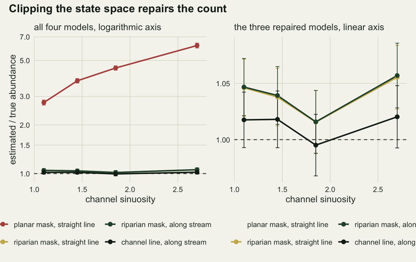
Sigma behaves the other way round. Both straight-line models, whatever their state space, return the same shrunken value. The two along-stream models sit on the truth almost everywhere: 0.514 km at the straightest setting, which is 2.4 Monte Carlo standard errors above the true 0.50, then 0.498, 0.501 and 0.500 km. Those four are a consistency check on the code rather than a measurement, because both along-stream arms are the model that generated the data; the measurement is the pair that is not.
mean_chord <- function(omega, sep, ds = 0.002) {
  n_w <- 4
  s_arc <- seq(0, n_w * lambda_m + sep + 0.01, by = ds)
  ang   <- omega * cos(2 * pi * s_arc / lambda_m)
  x_pos <- c(0, cumsum((cos(ang[-1]) + cos(ang[-length(ang)])) / 2 * ds))
  y_pos <- c(0, cumsum((sin(ang[-1]) + sin(ang[-length(ang)])) / 2 * ds))
  k_off <- round(sep / ds); i0 <- seq_len(round(n_w * lambda_m / ds))
  sqrt((x_pos[i0 + k_off] - x_pos[i0])^2 + (y_pos[i0 + k_off] - y_pos[i0])^2)
}
moment_sigma <- function(omega, sigma) {
  sep <- seq(0.01, 5 * sigma, length.out = 120)
  wt  <- exp(-sep^2 / (2 * sigma^2))
  c2  <- vapply(sep, function(s) mean(mean_chord(omega, s)^2), 0)
  sqrt(sum(wt * c2) / sum(wt))
}
om_sweep   <- seq(0.05, 1.78, length.out = 26)
sweep_tab  <- data.frame(sinuosity = 1 / besselJ(om_sweep, 0),
                         sigma = vapply(om_sweep, moment_sigma, 0, sigma = sigma_true))
mom_at     <- vapply(omega_set, moment_sigma, 0, sigma = sigma_true)
shrink_obs <- vapply(seq_along(des), function(k) pick(1, k, "sigma"), 0) / sigma_true
slope_lo   <- (shrink_obs[1] - shrink_obs[2]) / (sinu_set[2] - sinu_set[1])
slope_hi   <- (shrink_obs[3] - shrink_obs[4]) / (sinu_set[4] - sinu_set[3])
agree_n    <- max(abs(vapply(seq_along(des), function(k) pick(3, k, "n_ratio"), 0) -
                      vapply(seq_along(des), function(k) pick(4, k, "n_ratio"), 0)))
agree_s    <- max(abs(vapply(seq_along(des), function(k) pick(3, k, "sigma"), 0) -
vapply(seq_along(des), function(k) pick(4, k, "sigma"), 0)))ggplot(grid_tab, aes(sinuosity, sigma, colour = model)) +
geom_hline(yintercept = sigma_true, linetype = "dashed",
colour = te_body, linewidth = 0.5) +
geom_line(data = sweep_tab, aes(sinuosity, sigma), inherit.aes = FALSE,
colour = te_body, linetype = "dotted", linewidth = 0.7) +
geom_errorbar(aes(ymin = sigma - 1.96 * sigma_se, ymax = sigma + 1.96 * sigma_se),
width = 0.04, linewidth = 0.4) +
geom_line(linewidth = 0.9) +
geom_point(size = 2.2) +
scale_colour_manual(values = c(te_rust, te_gold, te_forest, te_ink), name = NULL) +
labs(x = "channel sinuosity", y = "estimated sigma (km)",
title = "The range is set by the distance",
subtitle = "dotted grey: shrinkage predicted by the chord lengths alone") +
theme_datasheet() +
theme(legend.position = "bottom") +
guides(colour = guide_legend(nrow = 2))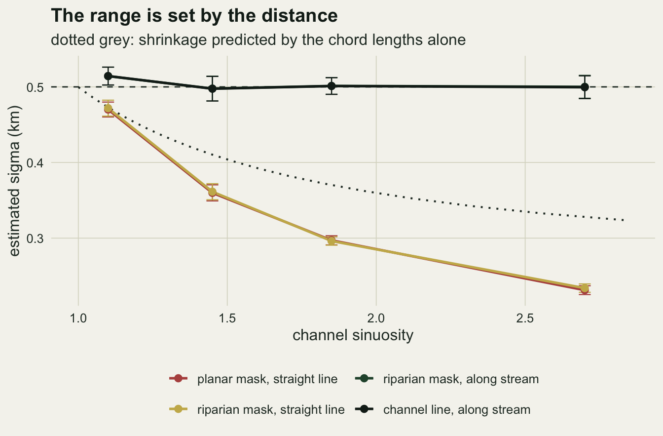
At the four sinuosities the straight-line fits return 0.94, 0.72, 0.59 and 0.46 of the true sigma. Whether that saturates depends on how the question is asked. Sigma keeps falling over the whole range and gives no sign of settling on a floor, but the fall per unit of sinuosity does flatten: 0.63 of sigma per unit between the first two settings against 0.16 between the last two. The damage therefore accumulates more slowly at high sinuosity without stopping, at this ratio of sigma to meander wavelength.
The dotted curve is a cheaper prediction that does not need the fit. Take the distribution of along-stream separations implied by the true detection function, replace each separation by the mean chord across it, and match second moments. That gives 0.473 km at the straightest setting and 0.328 km at the most sinuous, against fitted values of 0.470 and 0.231 km. The prediction has the right direction and the wrong size, and the gap widens with sinuosity. The reason is that the likelihood is not matching distances, it is explaining detections and non-detections together. On a tight bend a trap on the far limb sits a few hundred metres away as the crow flies and is almost always empty; the only way a straight-line model can account for an empty trap that close is to make sigma smaller still.
Why the inflation grows while the mask shrinks
The identity from the single survey does the bookkeeping. Abundance is the number detected times the state space divided by the effectively searched area, so writing the detected fraction as n / N gives a bias of (n / N) * (|S| / a_eff).
eff_tab <- do.call(rbind, lapply(seq_along(des), function(k) {
  g <- grid_raw[[k]]
  data.frame(sinuosity = sinu_set[k],
             mask = rep(c("planar mask", "riparian mask"), each = 2),
             part = rep(c("state space", "effectively searched"), 2),
             km2 = c(area_box[k], mean(g$aeff_box), area_rip[k], mean(g$aeff_rip)))
}))
box_ratio <- area_box / vapply(grid_raw, function(g) mean(g$aeff_box), 0)
rip_ratio <- area_rip / vapply(grid_raw, function(g) mean(g$aeff_rip), 0)
line_bias <- mean(vapply(seq_along(des), function(k) pick(4, k, "n_ratio"), 0))
box_pred  <- det_frac * box_ratio
rip_pred  <- det_frac * rip_ratio
box_gap   <- max(abs(box_pred - vapply(seq_along(des), function(k) pick(1, k, "n_ratio"), 0)))
aeff_true <- vapply(des, function(d) {
  pd <- 1 - exp(rowSums(n_occ * log1p(-pmin(p0_true *
          exp(-d$d_box^2 / (2 * sigma_true^2)), 1 - 1e-12))))
  sum(pd * d$w_box)
}, 0)
pred_true <- det_frac * area_box / aeff_true
For the planar mask the state space falls from 58.1 to 33.2 km2 as sinuosity rises, a factor of 1.75, while the effectively searched area falls from 17.9 to 4.6 km2, a factor of 3.92. The second factor is the larger, because the searched area is roughly the channel dressed in a band a couple of sigma wide and sigma is itself collapsing. Their ratio runs from 3.25 to 7.29, and multiplying by the detected fraction of 0.84 differs from the mean measured ratio by 0.07 at the sinuosity where the two are furthest apart, which is the gap between a mean of ratios and a ratio of means.
That splits the planar error in two. Holding sigma and p0 at their true values and recomputing a_eff over the same masks gives 17.3 km2 at the straightest setting and 10.9 km2 at the most sinuous, so the same identity would predict an inflation of 2.82 at the straightest setting and 2.57 at the most sinuous: flat, and if anything falling. Of the 3.92-fold collapse in the searched area, a factor of 1.59 is the mask geometry and the remaining 2.47 is the fitted sigma falling from 0.470 to 0.231 km. So the level of the planar error is a state-space error and all of its growth with sinuosity is the distance error, arriving through a_eff.
For the riparian mask the same ratio stays between 1.23 and 1.25. The strip is narrow enough that almost all of it is effectively searched, so the ratio is close to the reciprocal of the detected fraction and the two cancel. That cancellation is the reason a habitat mask alone repairs the count, and it is also the reason the repair is fragile: it depends on nearly every animal in the strip being catchable.
ggplot(eff_tab, aes(sinuosity, km2, colour = part)) +
  geom_line(linewidth = 0.9) +
  geom_point(size = 2.1) +
  facet_wrap(~ mask) +
  scale_x_continuous(expand = expansion(mult = 0.08)) +
  scale_y_log10() +
  scale_colour_manual(values = c(te_forest, te_rust), name = NULL) +
  labs(x = "channel sinuosity", y = "area (km2, log scale)",
       title = "The searched area collapses faster than the mask does",
       subtitle = "the abundance bias is the ratio of the two lines, times the detected fraction") +
  theme_datasheet() +
  theme(legend.position = "bottom")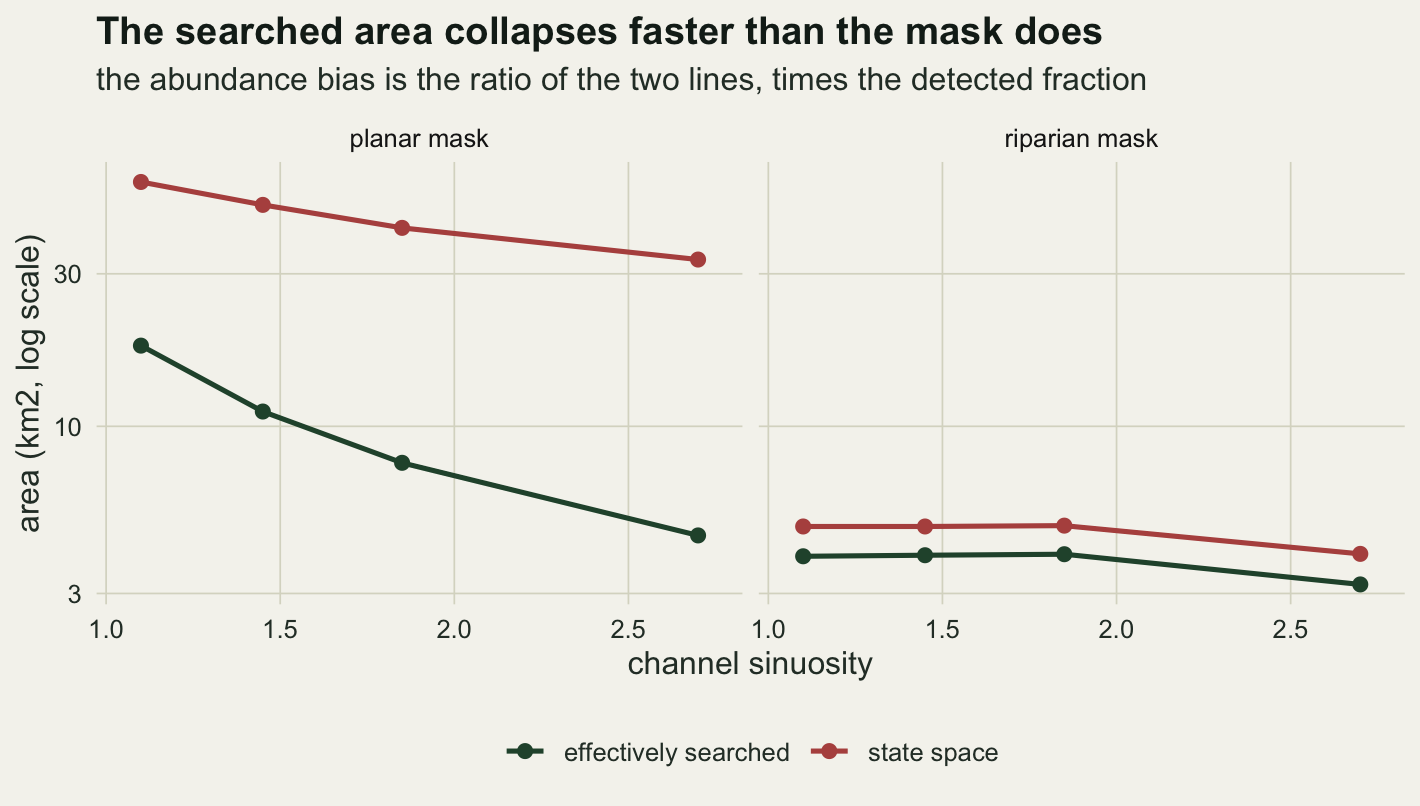
The mask repair needs the traps close together
Everything above uses traps every 250 m, which is half of sigma and much tighter than an SCR array on land would be. SCR sampling design and precision puts the precision optimum near two sigma on a plane. That optimum is measured at a fixed number of traps; here the length of the reach is fixed instead, so widening the spacing also removes traps, and the two arms are not directly comparable. If the riparian mask only fixes the count because detection is close to certain along the strip, widening the spacing should bring the bias back.
gap_set <- c(0.25, 0.5, 0.75, 1.25)
n_rep_gap <- 12
set.seed(88431)
gap_raw <- lapply(gap_set, function(gp) {
  d <- if (gp == 0.25) des[[3]] else build_design(omega_set[3], trap_gap = gp)
  run_cell(d, n_rep_gap, with_box = FALSE)
})
gap_tab <- do.call(rbind, lapply(seq_along(gap_set), function(i) {
  g <- gap_raw[[i]]
  data.frame(spacing = gap_set[i] / sigma_true,
             model = rep(c("riparian mask, straight line", "riparian mask, along stream",
                           "channel line, along stream"), each = 1),
             ratio = c(mean(g$N_rip / g$n_true), mean(g$N_ripn / g$n_true),
                       mean(g$N_line / g$n_true)),
             se = c(sd(g$N_rip / g$n_true), sd(g$N_ripn / g$n_true),
                    sd(g$N_line / g$n_true)) / sqrt(nrow(g)))
}))
gap_tab$model <- factor(gap_tab$model, levels = unique(gap_tab$model))
gap_det <- vapply(gap_raw, function(g) mean(g$n_det / g$n_true), 0)
gap_rip <- gap_tab$ratio[gap_tab$model == "riparian mask, straight line"]
gap_lin <- gap_tab$ratio[gap_tab$model == "channel line, along stream"]
gap_sig <- vapply(gap_raw, function(g) mean(g$s_line), 0)
gap_rn  <- gap_tab$ratio[gap_tab$model == "riparian mask, along stream"]
gap_pair <- lapply(gap_raw, function(g) (g$N_rip - g$N_line) / g$n_true)
gap_dif  <- vapply(gap_pair, mean, 0)
gap_dse  <- vapply(gap_pair, function(v) sd(v) / sqrt(length(v)), 0)
gap_ntrp <- vapply(gap_set, function(gp)
  length(seq(arc_buf, arc_buf + arc_trap, by = gp)), 0)
It does, and not only for the reason the mask is responsible for. At sinuosity 1.85, as trap spacing widens from 0.5 to 2.5 times sigma, the array thins from 37 traps to 19, 13 and 8, and the fraction of animals detected falls from 0.83 to 0.47. Effort and spacing move together here, which is the price of holding the reach fixed. The riparian mask with straight-line distance goes from 1.02 to 1.32 times the truth. The correctly specified channel line model also drifts, from 0.99 to 1.16, which is the ordinary sparse-array problem: at 2.5 sigma its own sigma has risen to 0.552 km against a truth of 0.50 and the array can no longer pin the detection scale down.
The part attributable to the distance metric is the gap between the two, and that gap widens steadily: 0.021 at half a sigma, 0.033 at one, 0.102 at one and a half, 0.168 at two and a half. All three models are fitted to the same capture histories at each spacing, so that difference is paired within replicate and its standard error is 0.0009, 0.0014, 0.0119 and 0.0371, much smaller than the separate bars in the figure below suggest: the two models in that difference are fitted to the same surveys, so most of the sampling error cancels. Switching the same riparian mask to along-stream distance closes most of the gap: its largest remaining difference from the correctly specified model across the four spacings is 0.023. So the habitat mask on its own is an adequate repair for abundance where detection along the reach is close to certain, and a partial one where it is not.
ggplot(gap_tab, aes(spacing, ratio, colour = model)) +
  geom_hline(yintercept = 1, linetype = "dashed", colour = te_body, linewidth = 0.5) +
  geom_errorbar(aes(ymin = ratio - 1.96 * se, ymax = ratio + 1.96 * se),
                width = 0.05, linewidth = 0.4) +
  geom_line(linewidth = 0.9) +
  geom_point(size = 2.2) +
  scale_colour_manual(values = c(te_gold, te_forest, te_ink), name = NULL) +
  labs(x = "trap spacing (units of sigma)", y = "estimated / true abundance",
       title = "Part of the repair, not all of it",
       subtitle = "sinuosity 1.85, twelve replicate surveys per point") +
  theme_datasheet() +
  theme(legend.position = "bottom") +
  guides(colour = guide_legend(nrow = 2))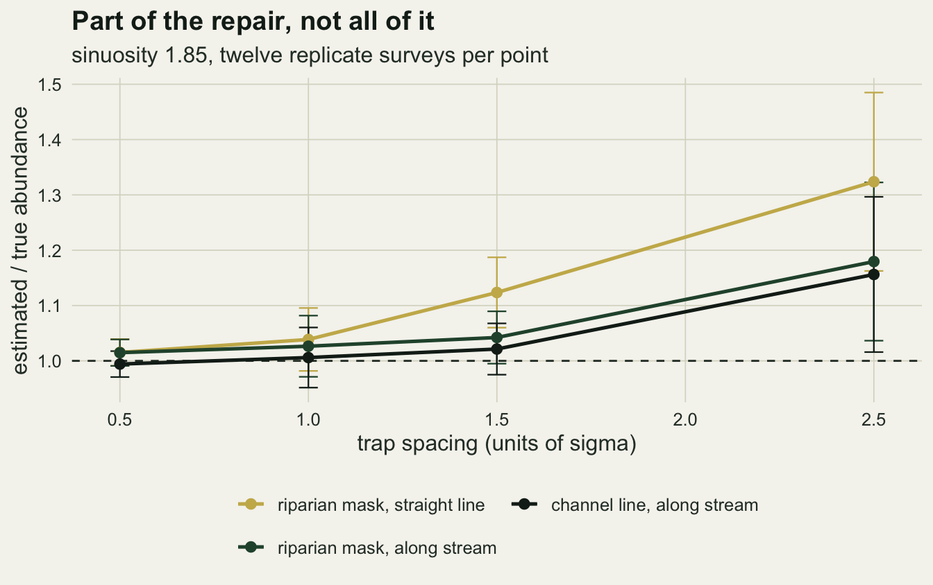
What to report
Report the state space as habitat, not as a buffer. A mask that is a rectangle or a disc around the traps is a claim that the animal could be anywhere in it, and on a stream that claim is false over most of the area. Clipping to the wetted channel plus whatever riparian width the species genuinely uses removed nearly all of the abundance error here, at every sinuosity, with no change to the distance metric. Give the mask area and the rule that produced it, because the estimated abundance is directly proportional to it.
Report sigma with the distance metric attached, and treat a sigma estimated on straight-line distance as a lower bound. The shrinkage measured here runs from 0.94 of the truth on a nearly straight reach to 0.46 at sinuosity 2.70, and it does not improve when the mask is clipped. Anything downstream of sigma inherits it: home range size, the 95 per cent activity radius, movement rates between reaches, and any connectivity statistic built from them.
Give the sinuosity of the study reach. It is one number, it is the ratio of channel length to valley length, and without it a reader cannot tell whether a straight-line analysis was nearly harmless or badly wrong. Sinuosity around 1.10 cost 6 per cent of sigma here and sinuosity 2.70 cost 54 per cent.
State the trap spacing in units of sigma alongside the mask. The cheap repair, a habitat mask with ordinary straight-line distances, sat 0.021 above the correctly specified model at half a sigma spacing and 0.168 above it at two and a half, on the paired comparison. A reader given the mask, the spacing and the sinuosity can work out for themselves how much of the analysis rests on the distance metric.
If sigma or anything derived from it is the quantity of interest, use the network. A 200 m riparian mask with along-stream distances and a one-dimensional channel state space agreed here to within 0.04 on the abundance ratio and 0.001 km on sigma at every sinuosity, which is a practical result: a narrow two-dimensional mask is available in general SCR software through a user-supplied distance function, and it does not force the analyst to argue that animals never leave the water.
Honest limits
The truth simulated here is one-dimensional. Activity centres sit on the channel and detection depends only on along-stream distance, so the one-dimensional model is correctly specified by construction and the riparian mask with along-stream distance is nearly so. Real stream animals use the bank, cross necks overland, and for some species a genuinely two-dimensional movement kernel with a strong network component would be the fairer description. Nothing here measures how the comparison changes when the truth is a mixture of the two, and that mixture is precisely the case where a modest riparian mask with a network distance should beat both extremes.
The planform is a single sine-generated wave of one wavelength. Real reaches change sinuosity along their length, carry tributaries, and have bends whose spacing is irregular, and a confluence adds a topology that no amount of bending produces. The tail-up post on this site works on a branching network, where the pairs of sites that are not flow-connected are the ones a straight line misjudges worst; everything above is meander only.
The sigma result is stated at one ratio of movement scale to meander wavelength. Sigma is 0.50 km against a wavelength of 1.5 km, one third. An animal whose movement scale is much shorter than the meander wavelength sees an almost straight channel and should lose much less; one whose scale spans several wavelengths sees a nearly straight valley and should also lose less, for the opposite reason. The monotone decline reported here belongs to this ratio, and a reader with a different one should rerun the sweep rather than read across.
Replication is 14 surveys per cell in the sinuosity grid and 12 in the spacing grid, which is enough for the means and their standard errors but not for interval coverage. Nothing above reports how often a Wald interval covers the truth, and for the planar model the question is not interesting anyway, since the point estimate is 2.7 to 6.2 times the truth. For the riparian and channel line models it is a real question and it is not answered here.
The estimator is the Poisson-N form throughout: activity centres are a Poisson process, abundance in the state space is D times its size, and nothing conditions on a fixed number of animals. Averaged over the four sinuosities the correctly specified channel line model sits 1.01 times the truth, a small upward bias that is the finite-sample behaviour of this estimator rather than a geometric effect, and it is the one place where a binomial-N formulation would be expected to behave differently. That comparison is not run here.
The detection model is half-normal with a constant p0, no behavioural response, no individual heterogeneity and no trap saturation. Baited traps in a stream have all four. Any of them would move the abundance estimates of every model in the comparison, and the mask and distance effects measured here would sit on top of that rather than replacing it.
Finally, the masks are discretised: 200 m cells for the planar mask, 100 m for the riparian strip and 25 m segments on the channel. The riparian strip is only four cells wide, so its area is the discretisation most at risk.
d3_fine <- build_design(omega_set[3], rip_cell = 0.05)
fit_fine <- fit_scr(caps_one, d3_fine$d_rip_e, d3_fine$w_rip,
                    one$n_true / sum(d3_fine$w_rip))
mesh_shift <- abs(fit_fine["abundance"] - fit_one["riparian_euc", "abundance"]) /
  fit_one["riparian_euc", "abundance"]
Halving that cell side to 50 m changes the riparian mask area from 4.89 to 4.87 km2 and moves the estimated abundance on the worked survey by 0.6 per cent, so the mesh is not carrying the result. A strip narrower than 200 m would need a finer mesh before its area could be trusted.
References
Efford MG 2004 Oikos 106(3):598-610 (10.1111/j.0030-1299.2004.13043.x)
Borchers DL, Efford MG 2008 Biometrics 64(2):377-385 (10.1111/j.1541-0420.2007.00927.x)
Royle JA, Chandler RB, Gazenski KD, Graves TA 2013 Ecology 94(2):287-294 (10.1890/12-0413.1)
Sutherland C, Fuller AK, Royle JA 2015 Methods in Ecology and Evolution 6(2):169-177 (10.1111/2041-210X.12316)
Leopold LB, Langbein WB 1966 Scientific American 214(6):60-70 (10.1038/scientificamerican0666-60)