---
title: "Home ranges in R: MCP versus kernel density"
description: "Estimate animal home ranges in R with minimum convex polygons and kernel density. Why the 100% MCP inflates with sample size and how bandwidth drives the KDE."
date: "2026-05-15 12:00"
categories: [R, MASS, home range, movement ecology, ecology tutorial]
image: thumbnail.png
image-alt: "A bilobed cloud of relocations with a 100% minimum convex polygon hull and 95% and 50% kernel density contours drawn over it."
---
A home range is the area an animal uses over some period. From a set of relocations (GPS fixes, VHF triangulations, resightings) the question is how to turn the point cloud into an area. Two estimators dominate the older literature and still anchor most workflows: the minimum convex polygon (MCP) and the kernel density estimator (KDE). They answer slightly different questions and they fail in different ways. This post builds both from base R plus `MASS`, starting on a synthetic bilobed range, and shows the two failure modes the estimators themselves carry: the MCP grows with sample size and chases outliers, while the KDE hands the whole result to one bandwidth choice.
## A synthetic range with two centres and a few excursions
Real ranges are rarely a single blob. We simulate 200 relocations from a mixture of two activity centres, then add six long excursions to stand in for the occasional foray outside the core. Coordinates are in kilometres and the data are illustrative, not a real site.
```{r}
#| label: setup
#| code-fold: true
#| code-summary: "Colours and plot theme used below"
#| results: hide
#| message: false
#| warning: false
te_ink <- "#16241d"; te_body <- "#2c3a31"; te_forest <- "#275139"
te_label <- "#46604a"; te_sage <- "#93a87f"; te_paper <- "#f5f4ee"
te_line <- "#dad9ca"; te_faint <- "#5d6b61"; te_gold <- "#cda23f"
te_green <- "#2f8f63"; te_red <- "#b5534e"
theme_te <- function(base_size = 12) {
  ggplot2::theme_minimal(base_size = base_size) +
    ggplot2::theme(
      text = ggplot2::element_text(colour = te_body),
      plot.title = ggplot2::element_text(colour = te_ink, face = "bold"),
      plot.subtitle = ggplot2::element_text(colour = te_faint),
      axis.title = ggplot2::element_text(colour = te_label),
      axis.text = ggplot2::element_text(colour = te_faint),
      panel.grid.major = ggplot2::element_line(colour = te_line, linewidth = 0.3),
      panel.grid.minor = ggplot2::element_blank(),
      plot.background = ggplot2::element_rect(fill = te_paper, colour = NA),
      panel.background = ggplot2::element_rect(fill = te_paper, colour = NA),
      legend.key = ggplot2::element_blank(),
      legend.title = ggplot2::element_text(colour = te_label),
      strip.text = ggplot2::element_text(colour = te_ink, face = "bold"))
}
```
```{r}
#| label: data
#| message: false
library(MASS); library(ggplot2); library(dplyr)

set.seed(4809)
n_core <- 200
comp <- rbinom(n_core, 1, 0.40)
xA <- rnorm(sum(comp == 0), 0.0, 1.20); yA <- rnorm(sum(comp == 0), 0.0, 1.20)
xB <- rnorm(sum(comp == 1), 4.0, 0.90); yB <- rnorm(sum(comp == 1), 2.5, 0.90)
core <- data.frame(x = c(xA, xB), y = c(yA, yB))

n_exc <- 6
ang <- runif(n_exc, 0, 2 * pi); rad <- runif(n_exc, 7, 10)
exc <- data.frame(x = 2 + rad * cos(ang), y = 1 + rad * sin(ang))

loc <- rbind(core, exc)
loc$kind <- c(rep("relocation", n_core), rep("excursion", n_exc))
nrow(loc)
```
## Minimum convex polygon
The MCP is the smallest convex polygon that contains a chosen fraction of the relocations. The 100% version is just the convex hull of every point; `chull` returns the hull vertices and the shoelace formula turns them into an area.
```{r}
#| label: mcp
mcp_area <- function(x, y) {
  h <- chull(x, y); xh <- x[h]; yh <- y[h]
  0.5 * abs(sum(xh * c(yh[-1], yh[1]) - c(xh[-1], xh[1]) * yh))
}
a100 <- mcp_area(loc$x, loc$y)

# 95% MCP: drop the 5% of points farthest from the centroid
cx <- mean(loc$x); cy <- mean(loc$y)
d2 <- (loc$x - cx)^2 + (loc$y - cy)^2
keep <- d2 <= quantile(d2, 0.95)
a95mcp <- mcp_area(loc$x[keep], loc$y[keep])

round(c(mcp100 = a100, mcp95 = a95mcp, ratio = a100 / a95mcp), 2)
```
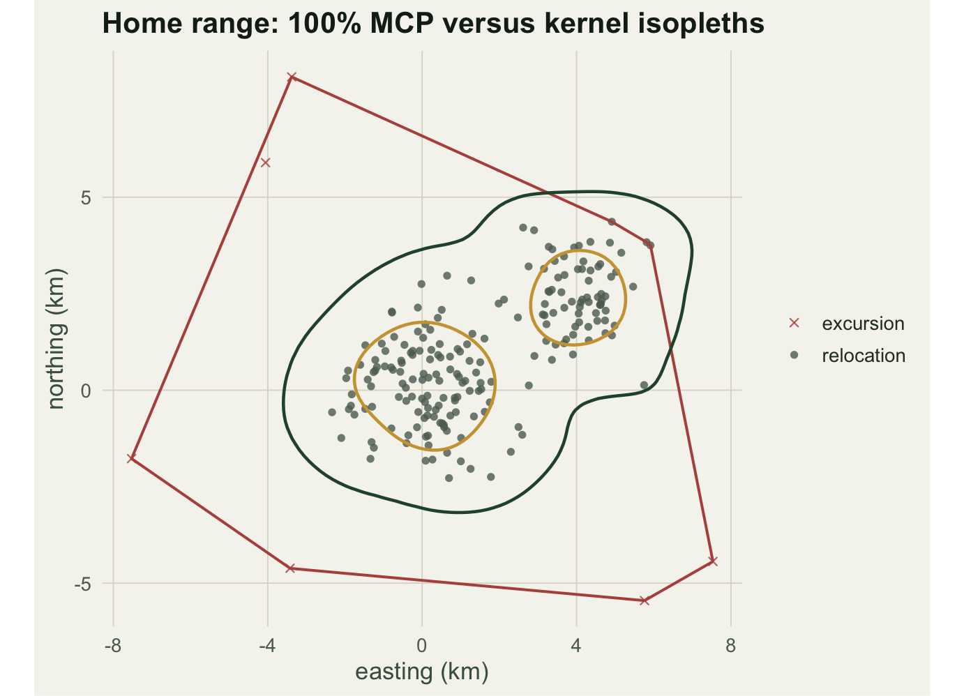
The 100% hull covers 136.5 km squared; dropping the peripheral 5% cuts it to 35.6 km squared. A factor of almost four separates them, and the six excursions drive the gap. That sensitivity to a handful of extreme fixes is the first problem with the MCP: the estimate is defined by its most peripheral points, so one long foray can double the reported range. The 95% rule trims that, but the 5% threshold is a convention with no biological content.
## The MCP grows with the number of relocations
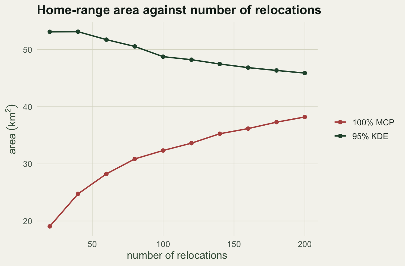
The deeper problem is subtler. Because the convex hull can only ever expand as points are added, MCP area increases with sample size and does not settle to a stable value. We subsample the core relocations at increasing sizes and average the area over 60 random draws at each size, then do the same for a 95% kernel range for comparison.
```{r}
#| label: accumulation
iso_threshold <- function(z, cell, p) {
  zv <- sort(as.vector(z), decreasing = TRUE)
  zv[which(cumsum(zv) * cell >= p)[1]]
}
iso_area <- function(z, cell, p) sum(z >= iso_threshold(z, cell, p)) * cell

set.seed(7788)
ns <- seq(20, n_core, by = 20); R <- 60
xlim0 <- range(core$x) + c(-1, 1) * 2; ylim0 <- range(core$y) + c(-1, 1) * 2
acc <- lapply(ns, function(nn) {
  am <- ak <- numeric(R)
  for (r in seq_len(R)) {
    s <- core[sample(nrow(core), nn), ]
    am[r] <- mcp_area(s$x, s$y)
    kk <- kde2d(s$x, s$y, n = 80, lims = c(xlim0, ylim0))
    cc <- diff(kk$x[1:2]) * diff(kk$y[1:2])
    ak[r] <- iso_area(kk$z, cc, 0.95)
  }
  data.frame(n = nn, mcp = mean(am), kde = mean(ak))
})
acc <- do.call(rbind, acc)
round(c(mcp_n20 = acc$mcp[1], mcp_n200 = acc$mcp[10],
        kde_n20 = acc$kde[1], kde_n200 = acc$kde[10]), 1)
# Second arm, on exactly the same subsamples: re-seeding replays the draws
# above, but now the bandwidth is held at the full-sample value instead of
# being recomputed inside each subsample.
h_full <- c(bandwidth.nrd(core$x), bandwidth.nrd(core$y))
set.seed(7788)
fixed_bw <- lapply(ns, function(nn) {
  af <- hx <- numeric(R)
  for (r in seq_len(R)) {
    s <- core[sample(nrow(core), nn), ]
    hx[r] <- bandwidth.nrd(s$x)
    kk <- kde2d(s$x, s$y, n = 80, lims = c(xlim0, ylim0), h = h_full)
    cc <- diff(kk$x[1:2]) * diff(kk$y[1:2])
    af[r] <- iso_area(kk$z, cc, 0.95)
  }
  data.frame(n = nn, kde_fix = mean(af), h_x = mean(hx))
})
fixed_bw <- do.call(rbind, fixed_bw)
acc$kde_fix <- fixed_bw$kde_fix; acc$h_x <- fixed_bw$h_x

data.frame(n = acc$n, kde = round(acc$kde, 1),
           kde_fix = round(acc$kde_fix, 1), h_x = round(acc$h_x, 2))
round(c(h_ratio = acc$h_x[10] / acc$h_x[1], nrd_rule = 10^(-1 / 5)), 3)
```
From 20 to 200 relocations the mean MCP area climbs from 19.1 to 38.2 km squared, a doubling with no sign of levelling off. The kernel range moves the other way, from 53.1 to 45.9 km squared, but that fall belongs to the bandwidth rule rather than to the estimator. `bandwidth.nrd` scales as the sample size to the power minus one fifth, so it shrinks as fixes accumulate: on the x axis it drops from 4.71 at 20 relocations to 3.15 at 200, a ratio of 0.669 against the 0.631 that rule predicts for a ten-fold change in n. Hold the bandwidth at the full-sample value and the kernel area rises with sample size as well, from 37.9 to 45.9 km squared, flattening out beyond about 80 relocations while the hull keeps climbing.
The contrast that survives is narrower than it first looks: the kernel estimate has a limit where the MCP does not, but over this window it is still drifting down, and it drifts because the selector trades bandwidth against sample size, not because the estimator is indifferent to effort. This is why MCP areas from studies with different tracking effort are not comparable: more fixes mean a larger reported range, all else equal. Reviews of home-range methods have made this point repeatedly (Harris 1990; Powell 2000).
```{r}
#| label: fig-accumulation
#| fig-cap: "Mean home-range area against the number of relocations, averaged over 60 random subsamples. The 100% MCP keeps climbing; the kernel range falls only while the bandwidth is recomputed inside each subsample, and rises when it is held at the full-sample value."
#| fig-alt: "Three lines against sample size: the red MCP line rises steadily from about 19 to 38, the dark green kernel line with a bandwidth recomputed inside each subsample drifts down from about 53 to 46, and the gold fixed-bandwidth kernel line rises from about 38 to 46 and flattens, meeting the green line at 200 relocations."
#| fig-width: 7
#| fig-height: 4.6
lev <- c("100% MCP", "95% KDE, bandwidth per subsample", "95% KDE, fixed bandwidth")
acc_long <- rbind(
  data.frame(n = acc$n, area = acc$mcp, estimator = lev[1]),
  data.frame(n = acc$n, area = acc$kde, estimator = lev[2]),
  data.frame(n = acc$n, area = acc$kde_fix, estimator = lev[3]))
acc_long$estimator <- factor(acc_long$estimator, levels = lev)
ggplot(acc_long, aes(n, area, colour = estimator)) +
  geom_line(linewidth = 0.8) + geom_point(size = 1.8) +
  scale_colour_manual(
    values = setNames(c(te_red, te_forest, te_gold), lev), name = NULL) +
  labs(title = "Home-range area against number of relocations",
       x = "number of relocations", y = expression(area ~ (km^2))) +
  theme_te(13)
```
## Kernel density and volume-based isopleths
The KDE replaces the hard hull with a smooth utilisation distribution: a density surface over the plane, estimated by placing a kernel on each relocation and summing. `MASS::kde2d` does this on a grid, and by default it picks a bandwidth from the normal reference rule for each axis.
```{r}
#| label: kde
xr <- range(loc$x) + c(-1, 1) * 2; yr <- range(loc$y) + c(-1, 1) * 2
href <- c(bandwidth.nrd(loc$x), bandwidth.nrd(loc$y))
k <- kde2d(loc$x, loc$y, n = 120, lims = c(xr, yr), h = href)
cell <- diff(k$x[1:2]) * diff(k$y[1:2])
round(c(h_x = href[1], h_y = href[2], integral = sum(k$z) * cell), 3)
```
To get a home range from a density surface you take an isopleth: the contour enclosing a given share of the total volume. The 95% isopleth is the smallest region holding 95% of the utilisation, and the 50% isopleth marks the core. Sort the grid densities from high to low, accumulate their volume, and read off the density level where the running total crosses the target.
```{r}
#| label: isopleth
thr95 <- iso_threshold(k$z, cell, 0.95); thr50 <- iso_threshold(k$z, cell, 0.50)
a95kde <- iso_area(k$z, cell, 0.95); a50kde <- iso_area(k$z, cell, 0.50)
round(c(kde95 = a95kde, kde50 = a50kde), 2)
```
The 95% kernel range is 59.5 km squared and the 50% core is 13.9 km squared. Unlike the convex hull, the kernel surface can represent the gap between the two centres and the separate cores, which a single polygon cannot.
```{r}
#| label: fig-overlay
#| fig-cap: "Relocations with the 100% MCP hull (red), the 95% kernel isopleth (green) and the 50% core (gold). Crosses mark the six excursions that stretch the hull."
#| fig-alt: "A bilobed cloud of relocation points with a red convex-polygon outline reaching out to scattered excursion crosses, a green kernel contour around both lobes, and gold contours on the two dense centres."
#| fig-width: 7.2
#| fig-height: 5.2
hull_idx <- chull(loc$x, loc$y)
hull_df  <- loc[c(hull_idx, hull_idx[1]), c("x", "y")]
grid_df  <- expand.grid(x = k$x, y = k$y); grid_df$z <- as.vector(k$z)

ggplot() +
  geom_point(data = loc, aes(x, y, shape = kind, colour = kind), size = 1.6, alpha = 0.8) +
  geom_path(data = hull_df, aes(x, y), colour = te_red, linewidth = 0.7) +
  geom_contour(data = grid_df, aes(x, y, z = z), breaks = thr95, colour = te_forest, linewidth = 0.8) +
  geom_contour(data = grid_df, aes(x, y, z = z), breaks = thr50, colour = te_gold, linewidth = 0.8) +
  scale_colour_manual(values = c(relocation = te_faint, excursion = te_red), name = NULL) +
  scale_shape_manual(values = c(relocation = 16, excursion = 4), name = NULL) +
  coord_equal() +
  labs(title = "Home range: 100% MCP versus kernel isopleths",
       x = "easting (km)", y = "northing (km)") +
  theme_te(13)
```
## Bandwidth is the choice that matters
The kernel result is only as good as the bandwidth. The normal reference rule assumes a single roughly Gaussian blob, so for a multimodal range it tends to oversmooth: the surface spreads across the gap and the isopleth inflates. Scaling the reference bandwidth up and down shows how much rides on it.
```{r}
#| label: bandwidth
bw_area <- function(mult) {
  kk <- kde2d(loc$x, loc$y, n = 120, lims = c(xr, yr), h = href * mult)
  cc <- diff(kk$x[1:2]) * diff(kk$y[1:2])
  iso_area(kk$z, cc, 0.95)
}
round(sapply(c(0.6, 1.0, 1.5), bw_area), 2)
```
At 0.6 times the reference the 95% range is 45.2 km squared; at the reference it is 59.5; at 1.5 times it is 81.3. The estimate almost doubles across a plausible band of smoothing, with the data unchanged. This is the central trade-off: too small a bandwidth breaks the range into islands around individual fixes, too large a bandwidth smears it into one oversized blob. Least-squares cross-validation and plug-in selectors try to choose objectively, and their behaviour has been studied at length (Worton 1989; Seaman and Powell 1996), but no rule removes the judgement entirely.
## Duration sets the precision, not the fix count
Everything so far holds the relocations fixed and asks what an estimator makes of them. The schedule that produced them has a failure mode of its own, and it is the expensive one: collar battery and memory go on the fix interval, while the answer mostly depends on how long the collar stays on the animal. Consecutive positions are correlated, and the time constant of that correlation, tau, is roughly how long the animal takes to forget where it was. A fix taken well inside tau repeats most of what the previous one already said.
A two-dimensional Ornstein-Uhlenbeck process makes the argument checkable. The animal is pulled back towards a centre with time constant tau, and its stationary distribution is a bivariate normal with standard deviation sigma on each axis. Positions separated by an interval `dt` satisfy an exact update, `x_next = mu + exp(-dt / tau) * (x - mu) + sigma * sqrt(1 - exp(-2 * dt / tau)) * z`, so the simulated track carries no discretisation error at any fix interval, and one rule generates the schedule whether the collar fires every minute or once a week.
```{r}
#| label: ou-model
q95 <- qchisq(0.95, 2)
tau_h <- 6          # position autocorrelation time, hours
sigma_km <- 1.2     # stationary standard deviation per axis, km
area_true <- pi * q95 * sigma_km^2
range_diam <- 2 * sqrt(q95) * sigma_km

# exact OU update, run as a recursive filter on the deviations from the centre
ou_dev <- function(n, dt, tau, sigma) {
  aa <- exp(-dt / tau)
  as.numeric(stats::filter(rnorm(n, 0, sigma * sqrt(1 - aa^2)), aa,
                           method = "recursive", init = rnorm(1, 0, sigma)))
}
# the model's own target, estimated its own way: isotropic normal 95% area
area_norm <- function(x, y) {
  vx <- mean((x - mean(x))^2); vy <- mean((y - mean(y))^2)
  pi * q95 * (vx + vy) / 2
}
# expected area over true area for n fixes dt apart, from the discrete
# autocovariance rather than its long-track limit
ratio_exact <- function(n, dt, tau) {
  rho <- exp(-dt / tau); kk <- seq_len(n - 1)
  1 - (n + 2 * sum((n - kk) * rho^kk)) / n^2
}

set.seed(60481)
chk <- ou_dev(2e5, 0.25 * tau_h, tau_h, sigma_km)
chk_sd <- sd(chk); chk_acf <- cor(chk[-1], chk[-length(chk)])
round(c(sd_sim = chk_sd, sd_target = sigma_km, acf1_sim = chk_acf,
        acf1_target = exp(-0.25), area_true = area_true), 4)
```
The simulator returns the spread and the lag one correlation it was asked for, so the machinery is right. With tau at `r sprintf("%.0f", tau_h)` hours and sigma at `r sprintf("%.1f", sigma_km)` km, the true 95% area is `r sprintf("%.2f", area_true)` km squared and the range is `r sprintf("%.2f", range_diam)` km across.
Because the movement model is known, the target is known too, and the estimator can be matched to it: average the two coordinate variances taken about the sample mean, which is the isotropic form of the normal 95% ellipse. The full covariance version adds a cross term carrying a bias of its own, and this model is isotropic, so the simple form is the one to test theory against. What comes out is a statement about the schedule and not about the estimator: a short track has seen a small part of the range whatever you fit to it afterwards.
Two consequences follow in closed form. The first is bias. The mean of an OU track has variance `2 * sigma^2 * tau / T` once the track is long against tau, and the variance taken about that estimated mean falls short by exactly that much, so the expected area is `1 - 2 * tau / T` of the truth. The second is precision. Squared deviations of a Gaussian process decorrelate twice as fast as the positions do, which puts the coefficient of variation of one coordinate variance at `sqrt(2 * tau / T)`. The area averages the two coordinates, and under an isotropic model those two variances are independent, so averaging them halves the variance once more and leaves the coefficient of variation of the area at `sqrt(tau / T)`. Neither expression mentions the number of fixes.
The first sweep holds the interval at a quarter of tau and lengthens the track.
```{r}
#| label: ou-duration
boot_cv <- function(v, B = 400) {
  bs <- replicate(B, {u <- sample(v, length(v), TRUE); sd(u) / mean(u)})
  sd(bs)
}

set.seed(31607)
dt_base <- 0.25; R_rep <- 1000
tmult <- c(2, 5, 10, 25, 50, 100, 400)
dur <- lapply(tmult, function(tm) {
  nfix <- tm / dt_base
  a <- replicate(R_rep, area_norm(ou_dev(nfix, dt_base * tau_h, tau_h, sigma_km),
                                  ou_dev(nfix, dt_base * tau_h, tau_h, sigma_km)))
  rr <- a / area_true; cv <- sd(rr) / mean(rr)
  data.frame(t_tau = tm, n_fix = nfix, ratio = mean(rr), se = sd(rr) / sqrt(R_rep),
             asym = 1 - 2 / tm, exact = ratio_exact(nfix, dt_base * tau_h, tau_h),
             cv = cv, cv_se = boot_cv(rr), cv_asym = sqrt(1 / tm))
})
dur <- do.call(rbind, dur)
cv_gain <- dur$cv[6] / dur$cv[5]
cv_gain_se <- cv_gain * sqrt((dur$cv_se[6] / dur$cv[6])^2 + (dur$cv_se[5] / dur$cv[5])^2)
round(dur, 4)
```
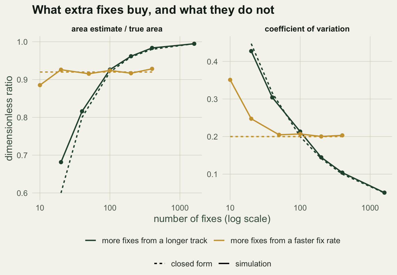
The design runs from `r sprintf("%.0f", min(tmult))` tau to `r sprintf("%.0f", max(tmult))` tau of tracking, `r sprintf("%.0f", R_rep)` replicate tracks each, and both closed forms hold over most of it. At `r sprintf("%.0f", dur$t_tau[4])` tau the mean area is `r sprintf("%.3f", dur$ratio[4])` of the truth with a Monte Carlo standard error of `r sprintf("%.3f", dur$se[4])`, against `r sprintf("%.3f", dur$asym[4])` from `1 - 2 * tau / T`; the coefficient of variation is `r sprintf("%.3f", dur$cv[4])` against `r sprintf("%.3f", dur$cv_asym[4])` from `sqrt(tau / T)`. At `r sprintf("%.0f", dur$t_tau[7])` tau the same pair reads `r sprintf("%.3f", dur$ratio[7])` against `r sprintf("%.3f", dur$asym[7])` and `r sprintf("%.4f", dur$cv[7])` against `r sprintf("%.4f", dur$cv_asym[7])`. The asymptotic bias formula breaks down at the short end, where it has to: at `r sprintf("%.0f", dur$t_tau[1])` tau it predicts an area of `r sprintf("%.1f", dur$asym[1])`, the simulation returns `r sprintf("%.3f", dur$ratio[1])`, and the exact discrete expression returns `r sprintf("%.3f", dur$exact[1])`. The square root law is the part worth carrying around: doubling the duration from `r sprintf("%.0f", dur$t_tau[5])` tau to `r sprintf("%.0f", dur$t_tau[6])` tau multiplies the coefficient of variation by `r sprintf("%.3f", cv_gain)`, standard error `r sprintf("%.3f", cv_gain_se)`, against the `r sprintf("%.3f", 1 / sqrt(2))` that halving the variance would give.
The second sweep holds the duration at `r sprintf("%.0f", dur$t_tau[4])` tau and moves the fix interval instead, from coarser than tau down to a sixteenth of it. The 100% MCP from the earlier section rides along on the same tracks.
```{r}
#| label: ou-interval
set.seed(90412)
dtm <- c(2.5, 1.25, 0.5, 0.25, 0.125, 0.0625); t_hold <- 25
pace <- lapply(dtm, function(dm) {
  nfix <- t_hold / dm; an <- am <- numeric(R_rep)
  for (r in seq_len(R_rep)) {
    xx <- ou_dev(nfix, dm * tau_h, tau_h, sigma_km)
    yy <- ou_dev(nfix, dm * tau_h, tau_h, sigma_km)
    an[r] <- area_norm(xx, yy); am[r] <- mcp_area(xx, yy)
  }
  rr <- an / area_true; cv <- sd(rr) / mean(rr)
  data.frame(dt_tau = dm, n_fix = nfix, ratio = mean(rr), se = sd(rr) / sqrt(R_rep),
             exact = ratio_exact(nfix, dm * tau_h, tau_h), cv = cv, cv_se = boot_cv(rr),
             mcp = mean(am), mcp_se = sd(am) / sqrt(R_rep))
})
pace <- do.call(rbind, pace)
fix_gain <- pace$cv[6] / pace$cv[5]
fix_gain_se <- fix_gain * sqrt((pace$cv_se[6] / pace$cv[6])^2 + (pace$cv_se[5] / pace$cv[5])^2)
mcp_gain <- pace$mcp[6] / pace$mcp[4]
mcp_gain_se <- mcp_gain * sqrt((pace$mcp_se[6] / pace$mcp[6])^2 + (pace$mcp_se[4] / pace$mcp[4])^2)
n_eff <- 1 / pace$cv[6]^2
z_share <- (pace$ratio[4] - dur$ratio[4]) / sqrt(pace$se[4]^2 + dur$se[4]^2)

# what T / tau independent relocations would give, for comparison
set.seed(41137)
iid <- replicate(R_rep, area_norm(rnorm(t_hold, 0, sigma_km), rnorm(t_hold, 0, sigma_km)))
iid_cv <- sd(iid) / mean(iid)
round(pace, 4)
```
The first two steps down are worth paying for, because sampling more coarsely than tau does throw information away: going from an interval of `r sprintf("%.2f", pace$dt_tau[1])` tau to `r sprintf("%.2f", pace$dt_tau[2])` tau drops the coefficient of variation from `r sprintf("%.3f", pace$cv[1])` to `r sprintf("%.3f", pace$cv[2])`, and the next step down, to `r sprintf("%.2f", pace$dt_tau[3])` tau, takes it to `r sprintf("%.3f", pace$cv[3])`. After that the dial stops working. Over the last eightfold increase in fixes, from `r sprintf("%.0f", pace$n_fix[3])` to `r sprintf("%.0f", pace$n_fix[6])` on the same length of track, the coefficient of variation reads `r sprintf("%.3f", pace$cv[3])`, `r sprintf("%.3f", pace$cv[4])`, `r sprintf("%.3f", pace$cv[5])` and `r sprintf("%.3f", pace$cv[6])`, and the final doubling of the fix rate multiplies it by `r sprintf("%.3f", fix_gain)` with a standard error of `r sprintf("%.3f", fix_gain_se)`, which is one. The mean area is flat across the same stretch, and the exact prediction is flat with it, at `r sprintf("%.3f", pace$exact[3])` and `r sprintf("%.3f", pace$exact[6])`. The two sweeps share the design point at `r sprintf("%.0f", t_hold)` tau with an interval of `r sprintf("%.2f", dt_base)` tau, measured twice under independent seeds, and the two values sit `r sprintf("%.2f", abs(z_share))` standard errors apart.
That flat column has a plain reading. A coefficient of variation of `r sprintf("%.3f", pace$cv[6])` off `r sprintf("%.0f", pace$n_fix[6])` fixes is what `r sprintf("%.1f", n_eff)` independent relocations would have delivered, and `r sprintf("%.0f", t_hold)` independent relocations do deliver `r sprintf("%.3f", iid_cv)` on the same estimator. The number of independent looks at the range is the duration in units of tau, `r sprintf("%.0f", t_hold)` here, and it takes no notice of how many rows the collar wrote. The MCP behaves as the earlier section said it would: at a fixed duration, quadrupling the fix rate from `r sprintf("%.0f", pace$n_fix[4])` to `r sprintf("%.0f", pace$n_fix[6])` fixes raises the mean hull area by a factor of `r sprintf("%.3f", mcp_gain)`, standard error `r sprintf("%.3f", mcp_gain_se)`, on tracking that contains no more information about the range than it did before.
```{r}
#| label: fig-fix-schedule
#| fig-cap: "Two ways of buying more fixes, plotted against the number of fixes on a log scale. Green: a longer track at a fixed interval of a quarter of tau. Gold: a faster fix rate over a fixed 25 tau of tracking. Dashed lines are the closed forms. The shortest track in the table is left out because the asymptotic bias formula is meaningless there."
#| fig-alt: "Two panels against the number of fixes on a log scale. In the left panel the green longer-track line climbs from about 0.68 to 0.99 times the true area, while the gold faster-fix-rate line starts near 0.89 and sits on a flat dashed line at 0.92 from then on. In the right panel the green coefficient of variation falls from about 0.43 to 0.05 along a dashed square-root curve, while the gold line drops twice and then runs flat at about 0.20."
#| fig-width: 7.2
#| fig-height: 5.0
arm <- c("more fixes from a longer track", "more fixes from a faster fix rate")
qn <- c("area estimate / true area", "coefficient of variation")
d2 <- dur[dur$t_tau >= 5, ]
sched <- rbind(
  data.frame(n_fix = d2$n_fix, value = d2$ratio, arm = arm[1], quantity = qn[1], src = "simulation"),
  data.frame(n_fix = d2$n_fix, value = d2$cv, arm = arm[1], quantity = qn[2], src = "simulation"),
  data.frame(n_fix = pace$n_fix, value = pace$ratio, arm = arm[2], quantity = qn[1], src = "simulation"),
  data.frame(n_fix = pace$n_fix, value = pace$cv, arm = arm[2], quantity = qn[2], src = "simulation"),
  data.frame(n_fix = d2$n_fix, value = d2$asym, arm = arm[1], quantity = qn[1], src = "closed form"),
  data.frame(n_fix = d2$n_fix, value = d2$cv_asym, arm = arm[1], quantity = qn[2], src = "closed form"),
  data.frame(n_fix = pace$n_fix, value = 1 - 2 / t_hold, arm = arm[2], quantity = qn[1], src = "closed form"),
  data.frame(n_fix = pace$n_fix, value = sqrt(1 / t_hold), arm = arm[2], quantity = qn[2], src = "closed form"))
sched$arm <- factor(sched$arm, levels = arm)
sched$quantity <- factor(sched$quantity, levels = qn)

ggplot(sched, aes(n_fix, value, colour = arm, linetype = src)) +
  geom_line(linewidth = 0.8) +
  geom_point(data = subset(sched, src == "simulation"), size = 1.8, show.legend = FALSE) +
  facet_wrap(~ quantity, scales = "free_y") +
  scale_x_log10() +
  scale_colour_manual(values = setNames(c(te_forest, te_gold), arm), name = NULL) +
  scale_linetype_manual(values = c(simulation = "solid", `closed form` = "22"), name = NULL) +
  guides(colour = guide_legend(order = 1), linetype = guide_legend(order = 2)) +
  labs(title = "What extra fixes buy, and what they do not",
       x = "number of fixes (log scale)", y = "dimensionless ratio") +
  theme_te(13) +
  theme(legend.position = "bottom", legend.box = "vertical",
        legend.margin = margin(0, 0, 0, 0))
```
This sits alongside the accumulation section rather than against it. That section resampled independent relocations and let their number grow, so its x axis was already an independent-fix count; this one holds the window fixed and lets the fixes crowd together inside it. Both find the hull inflating whenever the fix count rises, and they differ only in what a fix is worth: an independent relocation adds information, a fix taken inside tau mostly does not, so on a real collar the quantity that belongs on that earlier x axis is the duration in units of tau, not the number of rows in the file.
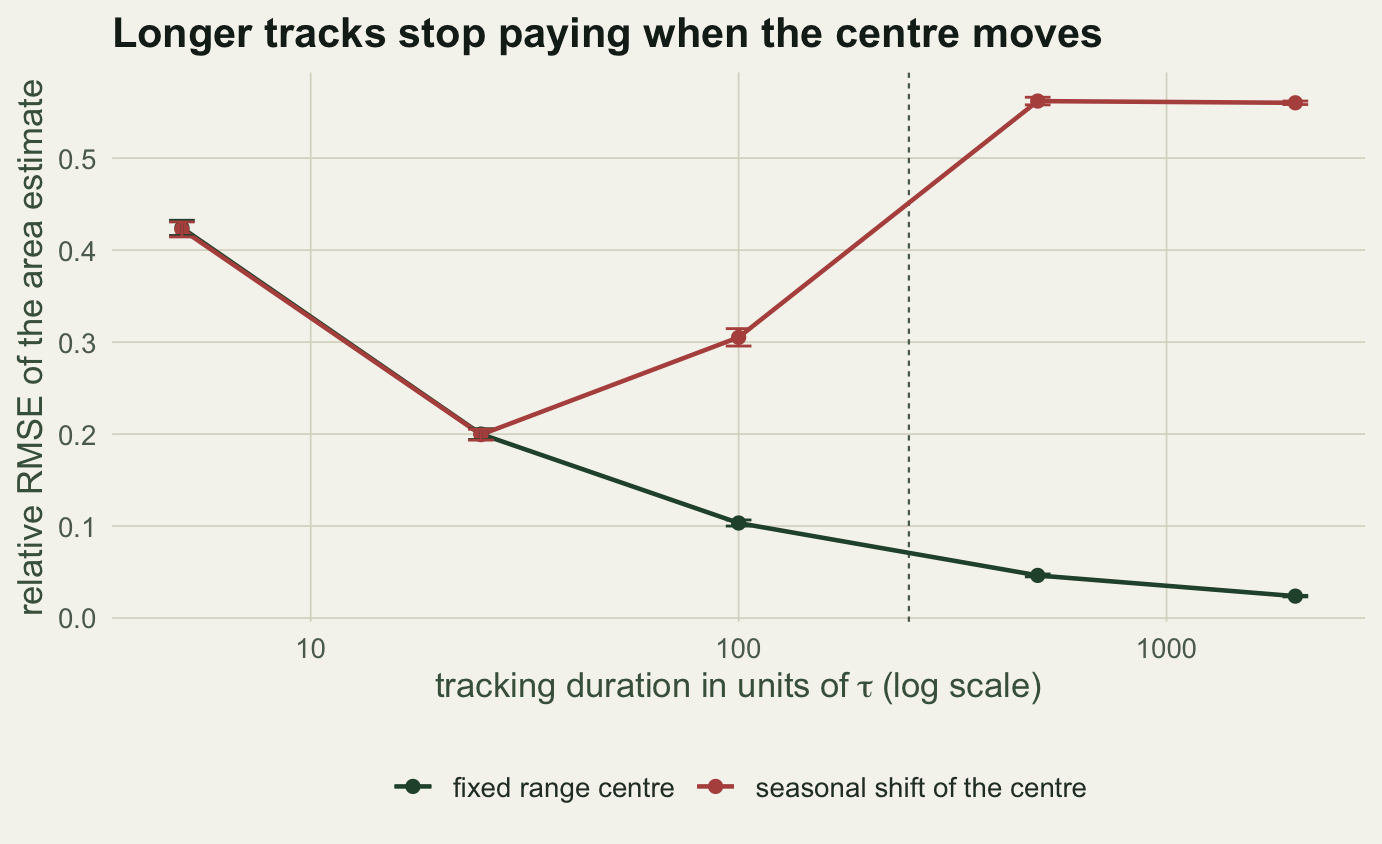
Now the hedge, and it is not a small one. All of the above assumes the range sits still. Let the centre drift and the recommendation reverses, because a longer track then answers a different question: the ground covered over a season rather than the area in use at any point within it. The same OU model gets a centre sliding along the x axis as an amplitude times `sin(2 * pi * t / P)`, the target stays the within-season area, and the score is relative root mean squared error against it.
```{r}
#| label: ou-season
set.seed(55231)
amp_km <- 1.5 * sigma_km; per_h <- 250 * tau_h; R_sea <- 400
tm_sea <- c(5, 25, 100, 500, 2000)
sea <- lapply(tm_sea, function(tm) {
  nfix <- tm / dt_base; dth <- dt_base * tau_h; tt <- seq_len(nfix) * dth
  ef <- es <- numeric(R_sea)
  for (r in seq_len(R_sea)) {
    xx <- ou_dev(nfix, dth, tau_h, sigma_km); yy <- ou_dev(nfix, dth, tau_h, sigma_km)
    ef[r] <- area_norm(xx, yy) / area_true - 1
    es[r] <- area_norm(xx + amp_km * sin(2 * pi * tt / per_h + runif(1, 0, 2 * pi)),
                       yy) / area_true - 1
  }
  data.frame(t_tau = tm, rmse_fix = sqrt(mean(ef^2)),
             se_fix = sd(ef^2) / (2 * sqrt(mean(ef^2)) * sqrt(R_sea)),
             rmse_sea = sqrt(mean(es^2)),
             se_sea = sd(es^2) / (2 * sqrt(mean(es^2)) * sqrt(R_sea)))
})
sea <- do.call(rbind, sea)
infl_pred <- amp_km^2 / (4 * sigma_km^2)
sea_worse <- sea$rmse_sea[5] / sea$rmse_fix[5]
swing_frac <- 2 * amp_km / range_diam
per_days <- per_h / 24
round(sea, 4)
```
The shift has an amplitude of `r sprintf("%.2f", amp_km)` km and a period of `r sprintf("%.1f", per_days)` days, which is `r sprintf("%.0f", per_h / tau_h)` tau; the centre swings back and forth over `r sprintf("%.0f", 100 * swing_frac)` per cent of the range diameter, so this is a seasonal drift and not a migration. Each of the `r sprintf("%.0f", R_sea)` replicate tracks per design starts at a random phase of the season. With the centre held still the error falls all the way along the grid, from `r sprintf("%.3f", sea$rmse_fix[1])` at `r sprintf("%.0f", sea$t_tau[1])` tau to `r sprintf("%.4f", sea$rmse_fix[5])` at `r sprintf("%.0f", sea$t_tau[5])` tau. With the centre drifting the two are indistinguishable up to `r sprintf("%.0f", sea$t_tau[2])` tau, `r sprintf("%.3f", sea$rmse_sea[2])` against `r sprintf("%.3f", sea$rmse_fix[2])` with standard errors of `r sprintf("%.3f", sea$se_sea[2])` and `r sprintf("%.3f", sea$se_fix[2])`, and after that the drift takes over: `r sprintf("%.3f", sea$rmse_sea[3])` at `r sprintf("%.0f", sea$t_tau[3])` tau, `r sprintf("%.3f", sea$rmse_sea[4])` at `r sprintf("%.0f", sea$t_tau[4])` tau and `r sprintf("%.3f", sea$rmse_sea[5])` at `r sprintf("%.0f", sea$t_tau[5])` tau, which is `r sprintf("%.0f", sea_worse)` times worse than a fixed-centre track of the same length. That last value is bias and not noise: a centre sweeping a sine wave adds a quarter of its squared amplitude to the average of the two coordinate variances, which predicts an inflation of `r sprintf("%.4f", infl_pred)` against the measured `r sprintf("%.4f", sea$rmse_sea[5])`, standard error `r sprintf("%.4f", sea$se_sea[5])`.
```{r}
#| label: fig-season-drift
#| fig-cap: "Relative RMSE of the area estimate against tracking duration, with a fixed range centre and with a centre that slides seasonally. The vertical line marks one seasonal period. The two curves lie on top of each other until the track is long enough to feel the drift."
#| fig-alt: "Relative RMSE against tracking duration on a log scale. The green fixed-centre curve falls steadily from about 0.42 to 0.02. The red seasonal-shift curve follows it down to a minimum of about 0.20 at 25 tau, then turns upwards and levels off near 0.56, crossing a vertical dashed line that marks one seasonal period."
#| fig-width: 7.2
#| fig-height: 4.4
lab <- c("fixed range centre", "seasonal shift of the centre")
sea_long <- rbind(
  data.frame(t_tau = sea$t_tau, rmse = sea$rmse_fix, se = sea$se_fix, model = lab[1]),
  data.frame(t_tau = sea$t_tau, rmse = sea$rmse_sea, se = sea$se_sea, model = lab[2]))
sea_long$model <- factor(sea_long$model, levels = lab)

ggplot(sea_long, aes(t_tau, rmse, colour = model)) +
  geom_vline(xintercept = per_h / tau_h, colour = te_faint, linetype = "22", linewidth = 0.4) +
  geom_line(linewidth = 0.8) + geom_point(size = 1.9) +
  geom_errorbar(aes(ymin = rmse - se, ymax = rmse + se), width = 0.06, linewidth = 0.5) +
  scale_x_log10() +
  scale_colour_manual(values = setNames(c(te_forest, te_red), lab), name = NULL) +
  labs(title = "Longer tracks stop paying when the centre moves",
       x = expression("tracking duration in units of" ~ tau ~ "(log scale)"),
       y = "relative RMSE of the area estimate") +
  theme_te(13) +
  theme(legend.position = "bottom")
```
So the advice is not to track for longer. It is to track for longer than the autocorrelation time and for less than whatever moves the range, and to say which period the estimate refers to. Of the durations on this grid the best under seasonal drift is `r sprintf("%.0f", sea$t_tau[which.min(sea$rmse_sea)])` tau, long enough for the sampling error to have come down and short enough for the drift not to have arrived; where that optimum falls depends on the amplitude and the period, and a wider swing moves it to the left. If the range shifts across the year, the honest product is one estimate per season with the duration reported alongside it, not one estimate per collar.
## Which to use
The MCP is quick, needs no tuning and is still the standard for a crude outer boundary, but its area depends on sample size and on the most extreme fixes, so it is a poor choice for comparing ranges across animals or studies with uneven effort. The KDE gives a proper utilisation distribution with a defensible core, handles multimodal ranges, and is far less sensitive to sample size, partly because the reference bandwidth rule shrinks as fixes accumulate and offsets the rise that remains at a fixed bandwidth, at the cost of a bandwidth decision that changes the answer. Report which estimator and, for the kernel, which bandwidth selector you used; without that, a home-range area is not reproducible. Both estimators also assume the relocations are an unbiased sample of use, which autocorrelated tracking data and gappy fix schedules can violate.
## References
Mohr 1947 American Midland Naturalist 37(1):223-249 (10.2307/2421652)
Worton 1989 Ecology 70(1):164-168 (10.2307/1938423)
Harris, Cresswell, Forde, Trewhella, Woollard & Wray 1990 Mammal Review 20(2-3):97-123 (10.1111/j.1365-2907.1990.tb00106.x)
Seaman & Powell 1996 Ecology 77(7):2075-2085 (10.2307/2265701)
Powell 2000, in Research Techniques in Animal Ecology (Boitani & Fuller, eds), Columbia University Press, ISBN 978-0-231-11341-2
Silverman 1986 Density Estimation for Statistics and Data Analysis, Chapman and Hall, ISBN 978-0-412-24620-3
## Related tutorials
- [Home-range overlap is not contact](../home-range-overlap-is-not-contact/)
- [Step lengths and turning angles](../step-lengths-turning-angles/)
- [Correlated random walks and net displacement](../correlated-random-walk/)
- [Classifying migrants from net squared displacement](../classifying-migration-from-displacement/)