library(ggplot2)
library(MASS)

te_paper  <- "#f5f4ee"
te_ink    <- "#16241d"
te_body   <- "#2c3a31"
te_forest <- "#275139"
te_rust   <- "#b5534e"
te_gold   <- "#c9b458"
te_line   <- "#dad9ca"

theme_datasheet <- function() {
  theme_minimal(base_size = 12) +
    theme(plot.background  = element_rect(fill = te_paper, colour = NA),
          panel.background = element_rect(fill = te_paper, colour = NA),
          panel.grid.major = element_line(colour = te_line, linewidth = 0.3),
          panel.grid.minor = element_blank(),
          strip.text       = element_text(colour = te_ink, face = "bold"),
          text             = element_text(colour = te_body),
          plot.title       = element_text(colour = te_ink, face = "bold"),
          plot.subtitle    = element_text(colour = te_body),
          axis.text        = element_text(colour = te_body))
}Home-range overlap is not contact
R
movement ecology
telemetry
permutation tests
disease ecology
simulation
ecology tutorial
Two collared animals can share one home range and meet rarely or often. Contact from paired GPS tracks in R, and why a time-shuffle test overstates it.
Two badgers in neighbouring setts carry GPS collars through one spring, and the question behind the collars is transmission: does the pair meet often enough to pass an infection? The first number anyone computes is the overlap of the two home ranges, and it comes back high. The kernel utilisation distributions sit almost on top of each other, the Bhattacharyya affinity is close to one, and the report says the two animals share their space. What the report cannot say from that number is whether they are ever in the same place at the same time. Overlap is a property of two maps. Contact is a property of two tracks read together, fix by fix.
This post makes that gap exact. Two animals are simulated on the same range with a movement model in which the marginal distribution of each animal does not depend on how their movements are coupled, so the home-range overlap is identical by construction at every level of coupling; that flatness is built in, not found. Simultaneous contact within a fixed distance then follows a closed form in the cross-correlation between the two tracks, which the simulation reproduces. None of this is new. Doncaster (1990) compared the distances between simultaneous fixes with the distances between all pairings of the two animals’ fixes, which is the contact the ranges alone would predict, and Long and colleagues (2014) examined eight indices of this kind of dynamic interaction and found that the ones built on a statistical test “are susceptible to Type I error, which increases at fine sampling resolutions”. The part that is measured here is that test: how far a test that shuffles the time order of one animal’s fixes overstates contact, what sets the size of the error, and whether a null that shifts one track in time instead of shuffling it keeps its level.
Several posts on this site stop short of the question. Home ranges in R: MCP versus kernel density estimates the range of one animal, and its section on duration uses the same Ornstein-Uhlenbeck model as below to show that the number of independent looks at a range is the tracking duration in units of the autocorrelation time, not the number of fixes; that is the fact the shuffle test forgets. Activity patterns and temporal overlap measures overlap in time of day between two species from camera traps, which says when both are active and nothing about whether they are in one place. Association indices for social networks builds contact from group sightings under the gambit of the group, where being seen together is the datum and no track exists. Co-occurrence is not interaction makes the same kind of argument about residual correlations between species, at the scale of sites rather than fixes. And Two-species point patterns: testing for interaction compares toroidal shift with random labelling for two mapped species; the circular time shift below is the same idea moved from the plane to the time axis, and it inherits the same weakness to a shared driver, which is discussed in the limits.
Two collars on one range
Each animal follows a two-dimensional Ornstein-Uhlenbeck process around the same centre, the standard model of a range-resident animal (Fleming and colleagues 2014 use it to separate movement at the scale of a step from movement at the scale of the range). Position on each axis is pulled back towards the centre with an autocorrelation time tau, measured here in fix intervals, and the stationary spread is sigma on each axis. Between consecutive fixes the exact update is x_next = a * x + sigma * sqrt(1 - a^2) * z with a = exp(-1 / tau), which stats::filter() runs as a recursive filter. The two animals are coupled through their innovations: animal B’s random kicks have correlation rho with animal A’s, and B’s starting position is drawn with the same correlation. Nothing else links them.
sig_rng <- 1
d_con   <- 0.5
n_fix   <- 1000
tau_one <- 5

sim_pair <- function(n, rho, tau, sig = sig_rng) {
  a_ar <- exp(-1 / tau)
  s_in <- sig * sqrt(1 - a_ar^2)
  z_a  <- matrix(rnorm(2 * n), n)
  z_b  <- rho * z_a + sqrt(1 - rho^2) * matrix(rnorm(2 * n), n)
  i_a  <- rnorm(2, 0, sig)
  i_b  <- rho * i_a + sqrt(1 - rho^2) * rnorm(2, 0, sig)
  run  <- function(z, i0) sapply(1:2, function(j)
    as.numeric(stats::filter(s_in * z[, j], a_ar, method = "recursive", init = i0[j])))
  list(A = run(z_a, i_a), B = run(z_b, i_b))
}
contact_frac <- function(A, B, d = d_con) mean(rowSums((A - B)^2) < d^2)
# stats::filter(method = "recursive") computes y[i] = x[i] + a * y[i - 1], with init as y[0]
stopifnot(isTRUE(all.equal(as.numeric(stats::filter(c(0.3, -1, 2), 0.5, method = "recursive",
                                                     init = 1)), c(0.8, -0.6, 1.7))))

set.seed(7301)
chk <- sim_pair(2e5, 0.6, tau_one)
chk_sd   <- sd(chk$A[, 1])
chk_acf  <- cor(chk$A[-1, 1], chk$A[-2e5, 1])
chk_rho  <- cor(chk$A[, 1], chk$B[, 1])
chk_lag  <- cor(chk$A[1:(2e5 - tau_one), 1], chk$B[(1 + tau_one):2e5, 1])
A long check run returns what the simulator was asked for: a positional standard deviation of 0.996 against sigma 1, a lag one autocorrelation of 0.818 against 0.819, a cross-correlation between the animals at the same fix of 0.602 against the rho of 0.6 it was given, and 0.218 at a lag of 5 fixes against 0.221.
That last pair of numbers is the whole mechanism. Because both animals share the pull strength a, the cross-covariance obeys C = a^2 * C + rho * sigma^2 * (1 - a^2) in the stationary state, so C = rho * sigma^2 at the same fix and rho * sigma^2 * exp(-k / tau) at a lag of k fixes. The marginal distribution of each animal is a bivariate normal with spread sigma whatever rho is. Two animals with rho of zero and two with rho of 0.9 have the same home ranges, and any overlap index computed from the true ranges takes its identical-ranges value in both cases (one for the Bhattacharyya affinity).
set.seed(7302)
show_n <- 300
trk <- do.call(rbind, lapply(c(0, 0.9), function(r_c) {
  p_s <- sim_pair(show_n, r_c, tau_one)
  hit <- rowSums((p_s$A - p_s$B)^2) < d_con^2
  lab <- sprintf("rho = %.1f: %d contacts in %d fixes", r_c, sum(hit), show_n)
  rbind(data.frame(x = p_s$A[, 1], y = p_s$A[, 2], animal = "A", hit = hit, panel = lab),
        data.frame(x = p_s$B[, 1], y = p_s$B[, 2], animal = "B", hit = hit, panel = lab))
}))
ggplot(trk, aes(x, y)) +
  geom_path(aes(colour = animal), linewidth = 0.35, alpha = 0.8) +
  geom_point(data = trk[trk$hit & trk$animal == "A", ], colour = te_rust, size = 1.3) +
  facet_wrap(~ panel) +
  coord_equal() +
  scale_colour_manual(values = c(A = te_forest, B = te_gold), name = "animal") +
  labs(x = "east (range standard deviations)", y = "north (range standard deviations)",
       title = "One range, two ways of sharing it") +
  theme_datasheet() +
  theme(legend.position = "bottom")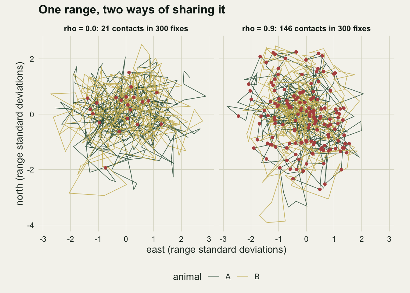
Contact follows the cross-correlation, overlap does not
Call the two animals in contact at a fix when they are closer than a distance d, here half a range standard deviation, and define the contact rate as the fraction of simultaneous fixes in contact. The difference between the two positions at one fix is bivariate normal with variance 2 * sigma^2 * (1 - rho) on each axis, so its squared length divided by that variance is chi-squared on two degrees of freedom, whose distribution function is 1 - exp(-x / 2). That gives the contact rate in closed form,
P(contact) = 1 - exp(-d^2 / (4 * sigma^2 * (1 - rho * exp(-k / tau)))),
with k = 0 for simultaneous fixes. At rho = 0 it is the contact that two independent animals on these ranges would have, which is also the rate Doncaster’s comparison computes from all pairings of fixes. For a contact distance small against the range the ratio of the two is 1 / (1 - rho): coupling multiplies contact without moving either range.
ba_kde <- function(A, B, h_bw = 1, n_grid = 60, lim = 4) {
  lims_g <- c(-lim, lim, -lim, lim)
  f_a <- kde2d(A[, 1], A[, 2], h = h_bw, n = n_grid, lims = lims_g)
  f_b <- kde2d(B[, 1], B[, 2], h = h_bw, n = n_grid, lims = lims_g)
  sum(sqrt(f_a$z * f_b$z)) * diff(f_a$x[1:2]) * diff(f_a$y[1:2])
}
closed_contact <- function(rho, k = 0, tau = tau_one, d = d_con, sig = sig_rng)
  1 - exp(-d^2 / (4 * sig^2 * (1 - rho * exp(-k / tau))))

rho_grid <- c(0, 0.2, 0.4, 0.6, 0.8, 0.9)
n_rep1   <- 150
n_shuf1  <- 20
lag_grid <- 0:15

set.seed(7303)
rho_out <- lapply(rho_grid, function(r_c) replicate(n_rep1, {
  p_s <- sim_pair(n_fix, r_c, tau_one)
  shuf <- mean(replicate(n_shuf1, contact_frac(p_s$A, p_s$B[sample.int(n_fix), ])))
  lagc <- sapply(lag_grid, function(k)
    contact_frac(p_s$A[1:(n_fix - k), , drop = FALSE], p_s$B[(1 + k):n_fix, , drop = FALSE]))
  c(obs = contact_frac(p_s$A, p_s$B), ba = ba_kde(p_s$A, p_s$B), exp_rng = shuf, lagc)
}))
rho_tab <- data.frame(
  rho     = rho_grid,
  obs     = sapply(rho_out, function(m_o) mean(m_o["obs", ])),
  obs_se  = sapply(rho_out, function(m_o) sd(m_o["obs", ]) / sqrt(n_rep1)),
  closed  = closed_contact(rho_grid),
  ba      = sapply(rho_out, function(m_o) mean(m_o["ba", ])),
  ba_se   = sapply(rho_out, function(m_o) sd(m_o["ba", ]) / sqrt(n_rep1)),
  exp_rng = sapply(rho_out, function(m_o) mean(m_o["exp_rng", ])),
  exp_se  = sapply(rho_out, function(m_o) sd(m_o["exp_rng", ]) / sqrt(n_rep1)))
gap_se   <- max(abs(rho_tab$obs - rho_tab$closed) / rho_tab$obs_se)
top_row  <- nrow(rho_tab)
ratio_hi <- rho_tab$obs[top_row] / rho_tab$exp_rng[top_row]
ratio_sm <- 1 / (1 - rho_grid[top_row])
ratio_cf <- closed_contact(rho_grid[top_row]) / closed_contact(0)
# a random re-pairing matches fix i of A with fix j of B with probability 1 / n,
# so its expected contact is the lagged formula averaged over all n^2 pairings
shuf_cf <- function(rho, n = n_fix) {
  k_all <- 0:(n - 1)
  w_k   <- ifelse(k_all == 0, n, 2 * (n - k_all))
  sum(w_k * closed_contact(rho, k = k_all)) / n^2
}
exp_cf    <- sapply(rho_grid, shuf_cf)
exp_z     <- max(abs(rho_tab$exp_rng - exp_cf) / rho_tab$exp_se)
ratio_cf2 <- closed_contact(rho_grid[top_row]) / exp_cf[top_row]

lag_hi  <- rho_out[[top_row]][-(1:3), ]
lag_obs <- rowMeans(lag_hi)
lag_se  <- apply(lag_hi, 1, sd) / sqrt(n_rep1)
lag_cf  <- closed_contact(rho_grid[top_row], k = lag_grid)
lag_gap <- max(abs(lag_obs - lag_cf) / lag_se)
Across 6 values of rho, with 150 simulated pairs of 1000 fixes each and tau at 5 fixes, the simulated contact rate reproduces the closed form: it runs from 0.0610 at rho = 0 (formula 0.0606) to 0.4633 at rho = 0.9 (formula 0.4647), and the largest gap at any rho is 2.0 Monte Carlo standard errors. The lagged version holds too: at rho = 0.9, contact between A at one fix and B up to 15 fixes later stays within 1.2 standard errors of the formula with exp(-k / tau) in it. This is a check of the algebra, not a result.
The two range-based quantities do not follow. The contact expected from the ranges, estimated by re-pairing each track with 20 random shuffles of the other, stays between 0.0604 and 0.0618 across the sweep, so at rho = 0.9 the pair meets 7.5 times as often as its ranges predict; the small-distance limit 1 / (1 - rho) would say 10. Two things close that gap. The finite d brings the closed-form ratio of contact at rho = 0.9 to contact at rho = 0 down to 7.67. And a random re-pairing is not quite the uncoupled pair: it matches each fix of A with any fix of B, including the few a short lag away that still carry coupling, so its expected contact is the lagged formula averaged over all pairings of fixes. That average is 0.0606 at rho = 0 and 0.0619 at rho = 0.9, the shuffle means sit within 1.5 Monte Carlo standard errors of it at every rho, and with it in the denominator the closed-form ratio is 7.51. The Bhattacharyya affinity of the two kernel utilisation distributions, the overlap index Fieberg and Kochanny (2005) recommend for similarity of use, is 0.976 at rho = 0 and 0.989 at rho = 0.9. The true affinity is one at every rho; the estimate falls short because each kernel density is built from one finite, autocorrelated track, and it rises slightly with rho because two coupled tracks share their sampling noise and so their estimated ranges look more alike. Neither movement is on the scale of the contact rate.
ov_long <- rbind(
  data.frame(rho = rho_tab$rho, val = rho_tab$ba, se = rho_tab$ba_se,
             what = "range overlap (Bhattacharyya affinity)"),
  data.frame(rho = rho_tab$rho, val = rho_tab$exp_rng, se = rho_tab$exp_se,
             what = "contact expected from the ranges"),
  data.frame(rho = rho_tab$rho, val = rho_tab$obs, se = rho_tab$obs_se,
             what = "simultaneous contact"))
cf_line <- data.frame(rho = seq(0, 0.9, by = 0.01))
cf_line$val <- closed_contact(cf_line$rho)
ggplot(ov_long, aes(rho, val, colour = what)) +
  geom_line(data = cf_line, aes(rho, val), inherit.aes = FALSE,
            linetype = "dashed", colour = te_ink, linewidth = 0.5) +
  geom_errorbar(aes(ymin = val - 1.96 * se, ymax = val + 1.96 * se), width = 0.015) +
  geom_line(linewidth = 0.8) +
  geom_point(size = 2.2) +
  scale_colour_manual(values = c(te_gold, te_forest, te_rust), name = NULL) +
  scale_y_continuous(limits = c(0, 1)) +
  labs(x = "coupling between the two animals (rho)", y = "overlap index or contact rate",
       title = "Overlap stays put while contact climbs",
       subtitle = "dashed: closed-form contact probability") +
  guides(colour = guide_legend(ncol = 1)) +
  theme_datasheet() +
  theme(legend.position = "bottom")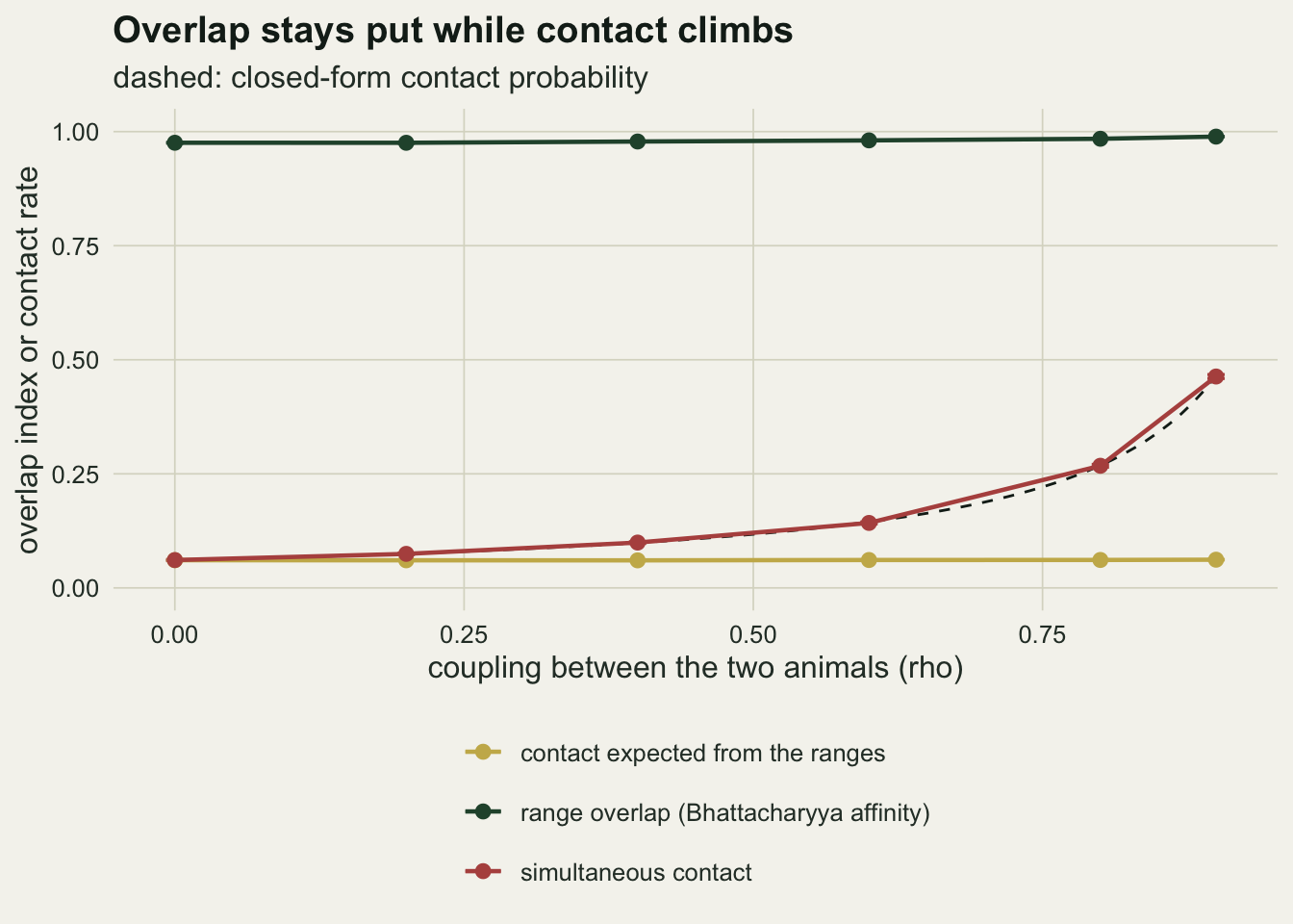
Testing for more contact than the ranges imply
The natural test takes the observed contact rate and asks whether it exceeds what the two ranges predict. Doncaster’s comparison uses all pairings of fixes with a significance test that treats fixes as independent; a Monte Carlo version of it, used below, shuffles the time order of B’s fixes and recomputes the contact rate many times. The shuffle keeps both ranges exactly and destroys any alignment in time, which is what a null for “no more contact than the ranges imply” should do. It also destroys the autocorrelation of each track, and that is where it goes wrong: a shuffled track is a set of independent draws from the range, so the null distribution it produces is as narrow as if every fix were an independent look.
The alternative keeps each track whole and slides B along the time axis by k fixes, wrapping the end of the track round to the start, which is the time version of the toroidal shift that Lotwick and Silverman (1982) introduced for mapped point patterns. Every shifted track has the autocorrelation of the real one and the same range. Shifts close to zero are excluded, because under coupling they still carry part of the correlation; here the excluded window is two autocorrelation times either side of zero, fixed before any run. Both tests use 99 null replicates and reject at the five per cent level.
n_null <- 99
m_mult <- 2

contact_idx <- function(A, B, idx, d = d_con) {
  dx <- A[, 1] - B[idx, 1]
  dy <- A[, 2] - B[idx, 2]
  colMeans(matrix(dx^2 + dy^2 < d^2, nrow(A)))
}
shift_set <- function(n, tau, n_draw) {
  m_ex <- ceiling(m_mult * tau)
  adm  <- m_ex:(n - m_ex)
  if (length(adm) > n_draw) sort(sample(adm, n_draw)) else adm
}
two_tests <- function(n, rho, tau, n_draw = n_null) {
  p_s  <- sim_pair(n, rho, tau)
  obs  <- contact_frac(p_s$A, p_s$B)
  perm <- contact_idx(p_s$A, p_s$B, replicate(n_draw, sample.int(n)))
  k_sh <- shift_set(n, tau, n_draw)
  sh   <- contact_idx(p_s$A, p_s$B, outer(0:(n - 1), k_sh, function(t, k) (t + k) %% n + 1))
  c(obs = obs, perm_var = var(perm), perm_mean = mean(perm),
    rej_perm  = (1 + sum(perm >= obs)) / (n_draw + 1) <= 0.05,
    rej_shift = (1 + sum(sh >= obs)) / (length(k_sh) + 1) <= 0.05,
    n_shift = length(k_sh))
}

set.seed(7304)
tau_show <- 20
p_show   <- sim_pair(n_fix, 0, tau_show)
obs_show <- contact_frac(p_show$A, p_show$B)
perm_show <- contact_idx(p_show$A, p_show$B, replicate(999, sample.int(n_fix)))
sh_show   <- contact_idx(p_show$A, p_show$B,
                         outer(0:(n_fix - 1), shift_set(n_fix, tau_show, 999),
                               function(t, k) (t + k) %% n_fix + 1))
sd_ratio_show <- sd(sh_show) / sd(perm_show)
p_perm_show <- (1 + sum(perm_show >= obs_show)) / (length(perm_show) + 1)
p_sh_show   <- (1 + sum(sh_show >= obs_show)) / (length(sh_show) + 1)
The figure shows both nulls for one uncoupled pair, with tau at 20 fixes and 1000 fixes per track; the display uses 999 replicates of each so that the shapes are visible. The pair has no coupling at all, and its observed contact rate is 0.036. The shifted tracks spread 1.8 times as widely as the shuffled ones (ratio of standard deviations). The shuffle gives this pair a p value of 0.993 and the shift gives 0.913. One pair is an illustration; the rates follow.
null_df <- rbind(data.frame(val = perm_show, null = "shuffled times"),
                 data.frame(val = sh_show,   null = "circular time shift"))
ggplot(null_df, aes(val, fill = null)) +
  geom_histogram(binwidth = 0.004, boundary = 0, position = "identity",
                 alpha = 0.6, colour = NA) +
  geom_vline(xintercept = obs_show, colour = te_ink, linewidth = 0.8) +
  scale_fill_manual(values = c("circular time shift" = te_forest,
                               "shuffled times" = te_rust), name = NULL) +
  labs(x = "contact rate under the null", y = "null replicates",
       title = "The shuffle forgets the autocorrelation",
       subtitle = "vertical line: the pair's observed contact rate") +
  theme_datasheet() +
  theme(legend.position = "bottom")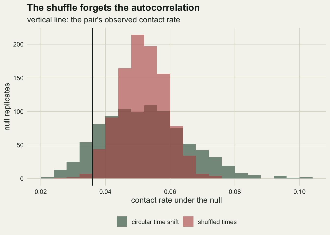
Which null keeps its level
The rates come from a sweep over tau and track length with no coupling, so every rejection is a false positive. Tau takes the values 1, 5, 20 and 50 fix intervals and the track length 250, 1000 and 3000 fixes. In field terms tau is the range crossing time divided by the fix interval: a collar that fixes every hour on an animal that takes about a day to cross its range sits near the tau of 20 and 50 end of this grid, and a collar that fixes once a day sits near the other end. The replication was fixed at 500 pairs per cell before the sweep ran.
tau_grid <- c(1, 5, 20, 50)
n_grid   <- c(250, 1000, 3000)
n_rep2   <- 500

set.seed(7305)
size_tab <- do.call(rbind, lapply(n_grid, function(n_c) do.call(rbind, lapply(tau_grid, function(t_c) {
  r_m <- replicate(n_rep2, two_tests(n_c, 0, t_c))
  o_c <- r_m["obs", ] - mean(r_m["obs", ])
  d_c <- r_m["obs", ] - r_m["perm_mean", ]
  data.frame(n = n_c, tau = t_c,
             perm  = mean(r_m["rej_perm", ]), shift = mean(r_m["rej_shift", ]),
             obs_var = mean(o_c^2),
             obs_var_se = sqrt((mean(o_c^4) - mean(o_c^2)^2) / n_rep2),
             cond_var = mean((d_c - mean(d_c))^2),
             cond_cor = cor(r_m["obs", ], r_m["perm_mean", ]),
             perm_var = mean(r_m["perm_var", ]),
             n_shift = min(r_m["n_shift", ]), cross = n_c / t_c)
}))))
mc_se   <- function(p) sqrt(p * (1 - p) / n_rep2)
se_nom  <- mc_se(0.05)
perm_hi <- size_tab[size_tab$tau == max(tau_grid), ]
perm_lo <- size_tab[size_tab$tau == min(tau_grid), ]
perm_20 <- size_tab[size_tab$tau == 20, ]
perm_5  <- size_tab[size_tab$tau == 5, ]
len_mult <- max(n_grid) / min(n_grid)
sh_bad  <- size_tab[which.min(size_tab$cross), ]
sh_ok   <- size_tab[-which.min(size_tab$cross), ]
sh_next <- min(sh_ok$cross)
sh_top  <- sh_ok[which.max(sh_ok$shift), ]
At the nominal level the Monte Carlo standard error of a rejection rate from 500 pairs is 0.0097. The shuffle holds its level only when the fixes are almost independent. At tau = 1 it rejects 0.040, 0.038 and 0.036 of true nulls at the three track lengths, a little under five per cent for a reason that comes up below. At tau = 5 the rates are already 0.076, 0.084 and 0.066; at tau = 20 they are 0.134, 0.148 and 0.140, and at tau = 50 they are 0.200, 0.238 and 0.234. A track 12 times longer does not bring the rate down. The error is set by the autocorrelation time in fix units, which fits what Long and colleagues saw as the sampling got finer: a shorter fix interval raises tau without adding independent looks at anything.
The circular shift holds its level in 11 of the 12 cells, down to a track 12.5 autocorrelation times long: its rejection rate there runs from 0.032 to 0.068, and the highest of those, at 1000 fixes and tau = 5, is 1.8 Monte Carlo standard errors above five per cent. It fails in the one cell where the excluded window takes most of the track: at 250 fixes and tau = 50, a track 5 autocorrelation times long, it rejects 0.176 of true nulls, against 0.200 for the shuffle. Two autocorrelation times either side of zero leave only 51 shifts, spanning 1 autocorrelation time, so they are nearly the same shifted track repeated, and their spread says nothing about how far an independent track could land from the observed one. The chunk below reruns that one cell on 1000 fresh uncoupled pairs with the window narrowed, down to excluding only the zero shift itself.
win_grid <- c(1, 10, 25, 50, ceiling(m_mult * sh_bad$tau))
n_rep5   <- 1000
set.seed(7308)
win_m <- replicate(n_rep5, {
  p_s <- sim_pair(sh_bad$n, 0, sh_bad$tau)
  obs <- contact_frac(p_s$A, p_s$B)
  sapply(win_grid, function(w) {
    k_w <- w:(sh_bad$n - w)
    sh  <- contact_idx(p_s$A, p_s$B, outer(0:(sh_bad$n - 1), k_w,
                                           function(t, k) (t + k) %% sh_bad$n + 1))
    (1 + sum(sh >= obs)) / (length(k_w) + 1) <= 0.05
  })
})
win_rate <- rowMeans(win_m)
win_se   <- sqrt(win_rate * (1 - win_rate) / n_rep5)
win_nsh  <- sh_bad$n - 2 * win_grid + 1
stopifnot(win_nsh[length(win_grid)] == sh_bad$n_shift)
Excluding only the zero shift, the same cell rejects 0.058 of true nulls with 249 shifts to compare against (Monte Carlo standard error 0.007, so 1.1 standard errors above five per cent). Starting the admitted shifts 10, 25 and 50 fixes from zero gives 0.074, 0.092 and 0.115, and starting them 100 fixes from zero, as the sweep did, gives 0.197 (standard errors up to 0.013). The rate climbs as the window widens: the failure comes from the window, not from the short track as such. A narrow window is not free, though. Under coupling a shift of k fixes keeps exp(-k / tau) of the cross-correlation, 0.98 of it at one fix here, so the shifts closest to zero carry part of the coupling into the null; how much power that costs was not measured.
size_long <- rbind(
  data.frame(size_tab[, c("n", "tau")], rate = size_tab$perm,  test = "shuffled times"),
  data.frame(size_tab[, c("n", "tau")], rate = size_tab$shift, test = "circular time shift"))
size_long$se <- mc_se(size_long$rate)
size_long$panel <- factor(sprintf("%d fixes", size_long$n),
                          levels = sprintf("%d fixes", n_grid))
ggplot(size_long, aes(tau, rate, colour = test)) +
  geom_hline(yintercept = 0.05, linetype = "dashed", colour = te_body, linewidth = 0.5) +
  geom_errorbar(aes(ymin = rate - 1.96 * se, ymax = rate + 1.96 * se), width = 0.08) +
  geom_line(linewidth = 0.8) +
  geom_point(size = 2.2) +
  facet_wrap(~ panel) +
  scale_x_log10(breaks = tau_grid) +
  scale_colour_manual(values = c("circular time shift" = te_forest,
                                 "shuffled times" = te_rust), name = NULL) +
  labs(x = "autocorrelation time tau (fix intervals)", y = "rejection rate with no coupling",
       title = "The shuffle's error grows with tau, not with the fix count") +
  theme_datasheet() +
  theme(legend.position = "bottom")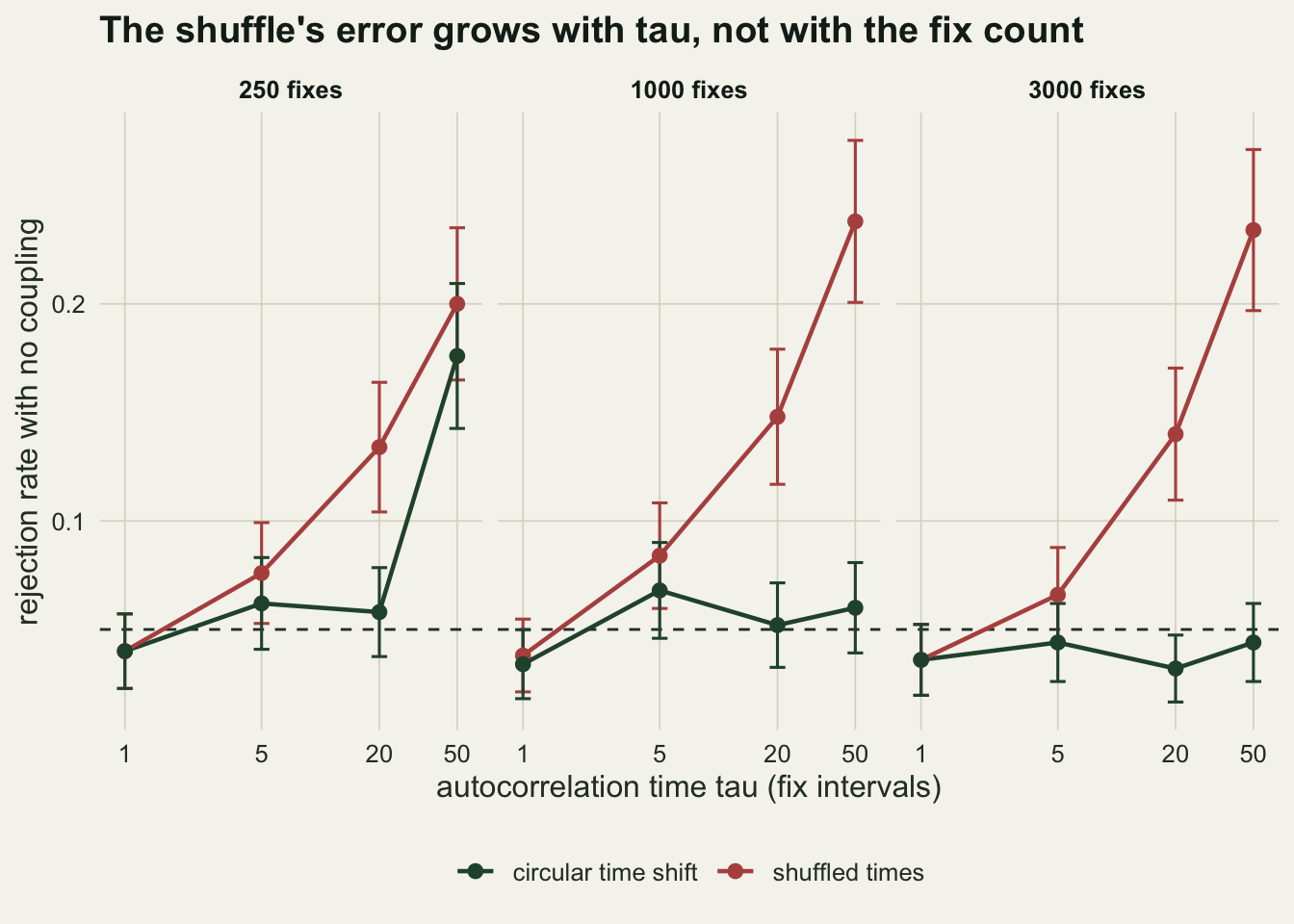
Why the shuffle fails: one variance ratio
The shuffle’s null has roughly the variance of a mean of n independent contact indicators, p * (1 - p) / n, with p the contact rate the ranges predict. The observed contact rate of an autocorrelated pair has that variance multiplied by an inflation factor, 1 + 2 * sum((1 - k / n) * c_k) / (p * (1 - p)), where c_k is the covariance between the contact indicators k fixes apart. With no coupling the difference between the two positions is itself an Ornstein-Uhlenbeck process with variance 2 * sigma^2 per axis and the same tau, so given the difference u at one fix, the difference k fixes later is normal around exp(-k / tau) * u, and the probability that both are in contact is a one-dimensional integral over u of a noncentral chi-squared probability. The chunk below computes the factor and compares it with the sweep, where the variance of the observed contact rate over the 500 uncoupled pairs of each cell, divided by p * (1 - p) / n, is the same quantity measured.
vif_closed <- function(tau, n, d = d_con, sig = sig_rng) {
  v_d  <- 2 * sig^2
  p_c  <- 1 - exp(-d^2 / (2 * v_d))
  k_mx <- min(n - 1, ceiling(40 * tau))
  c_k  <- sapply(seq_len(k_mx), function(k) {
    r_k <- exp(-k / tau)
    both <- integrate(function(u) (u / v_d) * exp(-u^2 / (2 * v_d)) *
                        pchisq(d^2 / (v_d * (1 - r_k^2)), df = 2,
                               ncp = r_k^2 * u^2 / (v_d * (1 - r_k^2))),
                      0, d, rel.tol = 1e-9)$value
    both - p_c^2
  })
  1 + 2 * sum((1 - seq_len(k_mx) / n) * c_k) / (p_c * (1 - p_c))
}
p_ind    <- closed_contact(0)
bin_var  <- p_ind * (1 - p_ind) / size_tab$n
size_tab$vif_cf  <- mapply(vif_closed, size_tab$tau, size_tab$n)
size_tab$vif_obs <- size_tab$obs_var / bin_var
size_tab$vif_z   <- (size_tab$obs_var - size_tab$vif_cf * bin_var) / size_tab$obs_var_se
size_tab$perm_rt <- size_tab$perm_var / bin_var
size_tab$size_nm <- 1 - pnorm(qnorm(0.95) / sqrt(size_tab$vif_cf))
size_tab$unc_rt  <- size_tab$obs_var / size_tab$perm_var
size_tab$cond_rt <- size_tab$cond_var / size_tab$perm_var
size_tab$size_cn <- 1 - pnorm(qnorm(0.95) / sqrt(size_tab$cond_rt))
vif_1000 <- size_tab[size_tab$n == 1000, ]
vif_z_mx <- size_tab[which.max(abs(size_tab$vif_z)), ]
nm_gap   <- size_tab$size_nm - size_tab$perm
gap_5    <- nm_gap[size_tab$tau == 5]
se_5     <- mc_se(size_tab$perm[size_tab$tau == 5])
long_tau <- size_tab$tau >= 20
cn_gap   <- size_tab$size_cn - size_tab$perm
The inflation factor at 1000 fixes is 1.02, 1.45, 3.80 and 8.87 at tau = 1, 5, 20 and 50, and it barely changes with track length. The measured ratios at the same four values are 1.00, 1.61, 3.37 and 9.18. Measured against the standard error of each measured variance, the largest of the 12 disagreements is 2.8 standard errors, at 3000 fixes and tau = 1, where the factor is 1.02 and the measured ratio 0.87. The shuffle’s own null variance, averaged over the pairs of a cell, stays between 0.87 and 0.97 times p * (1 - p) / n whatever tau is. So the shuffle’s null is narrower than the spread of the observed contact rate across pairs by about the square root of the inflation factor, and the factor is a function of tau: that part of the failure is arithmetic, and it is consistent with Long and colleagues’ finding, here for an Ornstein-Uhlenbeck pair and one test.
The rejection rate itself is not the arithmetic. Plugging the factor into a normal approximation, 1 - pnorm(qnorm(0.95) / sqrt(factor)), gives a rate above the measured one in 12 of the 12 cells. At tau = 1 the gap is the Monte Carlo p value itself: contact counts are integers, and a shuffled count equal to the observed one is counted against it. The chunk below repeats the tau = 1 test at 250 fixes on fresh pairs and scores each p value both ways.
n_rep4 <- 2000
set.seed(7307)
tie_m <- replicate(n_rep4, {
  p_s  <- sim_pair(min(n_grid), 0, min(tau_grid))
  obs  <- contact_frac(p_s$A, p_s$B)
  perm <- contact_idx(p_s$A, p_s$B, replicate(n_null, sample.int(min(n_grid))))
  c(ge  = (1 + sum(perm >= obs)) / (n_null + 1) <= 0.05,
    mid = (1 + sum(perm > obs) + 0.5 * sum(perm == obs)) / (n_null + 1) <= 0.05,
    tie = mean(perm == obs))
})
tie_rate <- rowMeans(tie_m)
tie_se   <- sqrt(tie_rate[1:2] * (1 - tie_rate[1:2]) / n_rep4)
Over 2000 pairs, 0.078 of the shuffled counts tie with the observed one. Counting ties against the observation, as the sweep does, the test rejects 0.036 of true nulls (standard error 0.004); counting them as half, it rejects 0.045 (standard error 0.005). At tau = 5 the gaps are 0.009, 0.002, 0.020 for the three track lengths, the largest of them 1.8 Monte Carlo standard errors. At tau = 20 and 50 they grow to between 0.051 and 0.087. Part of that is where the shuffle’s null is centred. Each pair’s shuffles are centred on that pair’s own range-expected contact, which rises and falls with its observed contact: over the 6 cells at tau = 20 and 50 the correlation between the two, across pairs, is between 0.41 and 0.66. The test compares the observed rate with that moving centre, and at 1000 fixes the variance of their difference is 2.95 and 7.42 times the shuffle’s own variance at tau = 20 and 50, against 3.57 and 9.82 for the observed rate alone. The normal approximation with the conditional ratio gives 0.169 and 0.273 in those two cells, against 0.199 and 0.290 from the factor and 0.148 and 0.238 measured; over the six cells the gap left is between 0.021 and 0.049, and that remainder is not closed form here. The inflation factor says which way the shuffle errs and why the error follows tau; the simulated rates above are the numbers.
What the correct null costs
A test that holds its level has to pay for it somewhere, and the circular shift pays in power, because an autocorrelated track has few independent looks at the other animal. The sweep below adds coupling at four levels for tracks of 1000 fixes at two autocorrelation times.
pow_rho <- c(0.1, 0.2, 0.3, 0.4)
pow_tau <- c(5, 20)
n_rep3  <- 250

set.seed(7306)
pow_tab <- do.call(rbind, lapply(pow_tau, function(t_c) do.call(rbind, lapply(pow_rho, function(r_c) {
  r_m <- replicate(n_rep3, two_tests(n_fix, r_c, t_c))
  data.frame(tau = t_c, rho = r_c, shift = mean(r_m["rej_shift", ]),
             perm = mean(r_m["rej_perm", ]), ratio = closed_contact(r_c) / closed_contact(0))
}))))
se_pow <- sqrt(0.25 / n_rep3)
pw5  <- pow_tab[pow_tab$tau == 5, ]
pw20 <- pow_tab[pow_tab$tau == 20, ]
stopifnot(all(pow_tab$perm > pow_tab$shift))
With 250 pairs per cell the Monte Carlo standard error of a power is at most 0.032. At rho = 0.2, a coupling that raises contact to 1.24 times what the ranges imply, the shift test detects it in 0.496 of pairs at tau = 5 and in 0.300 at tau = 20. At rho = 0.4 the rates are 0.972 and 0.744. The shuffle rejects more often in every one of these cells (at tau = 20: 0.500 at rho = 0.2), but part of that is the false positive rate measured above, 0.148 at the same tau and track length, so it is not power that can be compared. The same 1000 fixes carry less information about contact when tau is longer, and a test that admits this finds less.
What to report
Report home-range overlap and contact as two quantities, and do not let the first stand in for the second. For a question about transmission or social behaviour the quantity is the contact rate at a stated distance and a stated time window, next to the rate the two ranges alone predict; the ratio of those two measures the excess contact, and the overlap index says nothing about it.
State the autocorrelation time of the tracks in fix intervals whenever a test for excess contact is reported. If the collars fix at an interval well below the range crossing time, a test that shuffles fix times will find interaction in pairs that have none, and the rate climbs with the fix rate rather than falling. Any test whose null treats fixes as independent draws, a chi-squared test on counts of close and distant fixes among them, rests on the same variance and should be expected to fail the same way, although only the shuffle was run here. Report the null that was used, what it holds fixed, and the size of the excluded lag window for a shift null.
Use a null that keeps each track whole. The circular time shift, with a window of two autocorrelation times either side of zero, held its level here on every track at least 12.5 autocorrelation times long. On the track of 5 autocorrelation times that window left too few shifts, and excluding only the zero shift brought the rejection rate to 0.058, within Monte Carlo error of five per cent, at the price of letting short-lag coupling into the null. Report the window, and check by simulation the size it gives at the track length and tau at hand; a parametric null simulated from movement models fitted to each animal is the other option, a different test with assumptions of its own.
Honest limits
The movement model is the simplest range-resident one: two isotropic Ornstein-Uhlenbeck processes with a shared centre, the same tau and the same spread, coupled through their innovations. Real animals have ranges of different sizes that only partly overlap, and velocity autocorrelation at short lags that this model lacks. The closed form needs the shared tau and the shared spread; with unequal ranges the difference of positions is still normal, but its variance has more terms.
The circular shift is only valid if nothing else in the track depends on time. Two animals that both visit one waterhole at dusk will be in contact more often at simultaneous fixes than at shifted ones even with no attraction between them, because the shared daily rhythm is broken by any shift that is not a whole number of days. This is the time version of the shared gradient that defeats toroidal shift in the point pattern post, and it was not simulated here. Restricting shifts to whole days keeps the daily rhythm aligned, and it cuts the number of available shifts further.
The excluded window of two autocorrelation times was fixed before running. The window check above varied it only on the shortest track and only with no coupling; what a narrower window costs in power when the animals are coupled was not measured. The true tau is also used to set the window, where real work has to estimate it.
The contact distance is half a range standard deviation, which is large for direct transmission; for a small distance the closed form gives the coupling ratio 1 / (1 - rho), but a small d also makes contact rarer, and how the gap between the measured rejection rates and the normal approximation behaves then is open; no smaller d was run. Contact is counted only at simultaneous fixes; if contact is counted over all fix pairs within a time window, its rate is the lagged formula averaged over the window, which dilutes the coupling. Neither that nor missing or unsynchronised fixes was simulated.
References
Doncaster CP 1990 Journal of Theoretical Biology 143(4):431-443 (10.1016/S0022-5193(05)80020-7)
Long JA, Nelson TA, Webb SL, Gee KL 2014 Journal of Animal Ecology 83(5):1216-1233 (10.1111/1365-2656.12198)
Fieberg J, Kochanny CO 2005 Journal of Wildlife Management 69(4):1346-1359 (10.2193/0022-541X(2005)69[1346:QHOTIO]2.0.CO;2)
Fleming CH, Calabrese JM, Mueller T, Olson KA, Leimgruber P, Fagan WF 2014 The American Naturalist 183(5):E154-E167 (10.1086/675504)
Lotwick HW, Silverman BW 1982 Journal of the Royal Statistical Society Series B 44(3):406-413 (10.1111/j.2517-6161.1982.tb01221.x)