---
title: "Association indices for social networks"
description: "Turn group sightings into a weighted animal social network in R: the simple ratio and half-weight association indices by hand, and when the choice matters."
date: "2026-06-19 11:00"
date-modified: "2026-10-14"
categories: [R, social networks, animal behaviour, association index, ecology tutorial]
image: thumbnail.png
image-alt: "A node and link diagram of six individuals labelled A to F: three shaded one colour on the left and three another on the right, with edge width scaling with the association index and a single link bridging the two groups."
---
*Corrected 14 October 2026: the title of the scatter plot of the two indices still said they diverge for pairs seen apart, although the pairs seen apart most often sit at the origin with no gap; it now says the gap is widest at middling association.*
*Corrected 1 October 2026: the post said the gap between the half-weight and simple ratio indices keeps growing as single sightings grow relative to joint ones; it now says the gap is widest when the two are comparable and narrows again when single sightings dominate, as the pair table shows.*
You watch a marked population: a flock, a pod, a troop. Each time you go out you record who was seen together. Out of those sightings you want a network: a weight on every pair of individuals that says how strongly they associate. This first post builds that network from group sightings and shows why the arithmetic you pick to do it is a real decision, not a formality.
## The gambit of the group
Field data rarely record "A groomed B" or "A followed B". They record groups: a set of individuals seen together at one time. The usual move is to treat everyone in a group as associating with everyone else in it. That assumption has a name, the gambit of the group, and the whole network inherits it. It is a strong assumption and we return to it in the checking post; for now we take it and see how far it gets us.
So the raw material is a list of observations, each one an individual seen in a group at a sampling period. A period can hold more than one group (you might see two subgroups on the same morning). Here is a small hand-built example with six individuals across fifteen periods.
```{r}
#| label: setup
#| code-fold: true
#| code-summary: "Setup: packages, colours and plot theme"
#| results: hide
#| message: false
#| warning: false
library(ggplot2)
theme_set(theme_minimal(base_size = 12) +
  theme(plot.background = element_rect(fill = "#f5f4ee", colour = NA),
        panel.background = element_rect(fill = "#f5f4ee", colour = NA),
        panel.grid.minor = element_blank()))
knitr::opts_chunk$set(dev.args = list(bg = "#f5f4ee"))
```
```{r}
#| label: data
obs <- data.frame(
  period = c(1,1, 2,2, 3,3, 4,4,4, 5,5, 6,6, 7, 8,8, 9,9,9, 10,10,
             11,11, 12, 13,13, 14,14, 15),
  group  = c(1,1, 1,1, 1,1, 1,1,2, 1,1, 1,1, 1, 1,1, 1,1,2, 1,1,
             1,1, 1, 1,1, 1,1, 1),
  id     = c("A","B", "A","B", "A","B", "A","B","C", "A","C", "B","C", "A",
             "C","D", "A","B","C", "D","E", "D","E", "E", "E","F", "E","F","F")
)
ids <- sort(unique(obs$id))
n <- length(ids)
```
## Four counts per pair
For any pair of individuals the association index is a ratio, and the ratio needs four counts. Over the sampling periods, count how many times the pair was seen together, how many times both were seen but in different groups, and how many times only one of them was seen at all.
Writing the pair as $i$ and $j$:
- $x$: periods where $i$ and $j$ were in the **same** group.
- $y_{ab}$: periods where **both** were seen but in **different** groups.
- $y_a$: periods where **only** $i$ was seen.
- $y_b$: periods where **only** $j$ was seen.
The following function walks the periods and returns those four numbers for a pair.
```{r}
#| label: counts
counts <- function(i, j) {
  x <- yab <- ya <- yb <- 0L
  for (p in unique(obs$period)) {
    sub <- obs[obs$period == p, ]
    gi <- sub$group[sub$id == i]
    gj <- sub$group[sub$id == j]
    seen_i <- length(gi) > 0
    seen_j <- length(gj) > 0
    if (seen_i && seen_j) {
      if (any(gi %in% gj)) x <- x + 1L else yab <- yab + 1L
    } else if (seen_i) ya <- ya + 1L
    else if (seen_j) yb <- yb + 1L
  }
  c(x = x, yab = yab, ya = ya, yb = yb)
}
counts("A", "B")
```
## Two indices, one denominator apart
The simple ratio index (SRI) puts the together-count over every period where at least one of the pair was seen:
$$\text{SRI} = \frac{x}{x + y_{ab} + y_a + y_b}.$$
The half-weight index (HWI) keeps the same numerator but halves the weight on the periods where only one member was identified:
$$\text{HWI} = \frac{x}{x + y_{ab} + \tfrac{1}{2}(y_a + y_b)}.$$
The half-weight was built for a specific worry (Cairns and Schwager 1987): in many protocols, when two animals are together you are **less** likely to identify both of them than when they are apart. That bias inflates the single-identification counts $y_a$ and $y_b$, which drags the SRI down. Halving those counts pushes back against the bias. The gap between the two indices is widest where $y_a + y_b$ is comparable to $x + y_{ab}$; where single sightings far outnumber the together-count, both indices are small and the gap narrows again.
Let me compute both for every pair and store the two matrices.
```{r}
#| label: indices
sri <- hwi <- matrix(0, n, n, dimnames = list(ids, ids))
tab <- list()
for (a in 1:(n-1)) for (b in (a+1):n) {
  cc <- counts(ids[a], ids[b])
  s <- cc["x"] / (cc["x"] + cc["yab"] + cc["ya"] + cc["yb"])
  h <- cc["x"] / (cc["x"] + cc["yab"] + 0.5*(cc["ya"] + cc["yb"]))
  sri[ids[a], ids[b]] <- sri[ids[b], ids[a]] <- s
  hwi[ids[a], ids[b]] <- hwi[ids[b], ids[a]] <- h
  tab[[length(tab)+1]] <- data.frame(i = ids[a], j = ids[b],
      x = cc["x"], yab = cc["yab"], ya = cc["ya"], yb = cc["yb"],
      SRI = round(s, 3), HWI = round(h, 3), diff = round(h - s, 3))
}
tab <- do.call(rbind, tab); rownames(tab) <- NULL
tab[order(-tab$SRI), ]
```
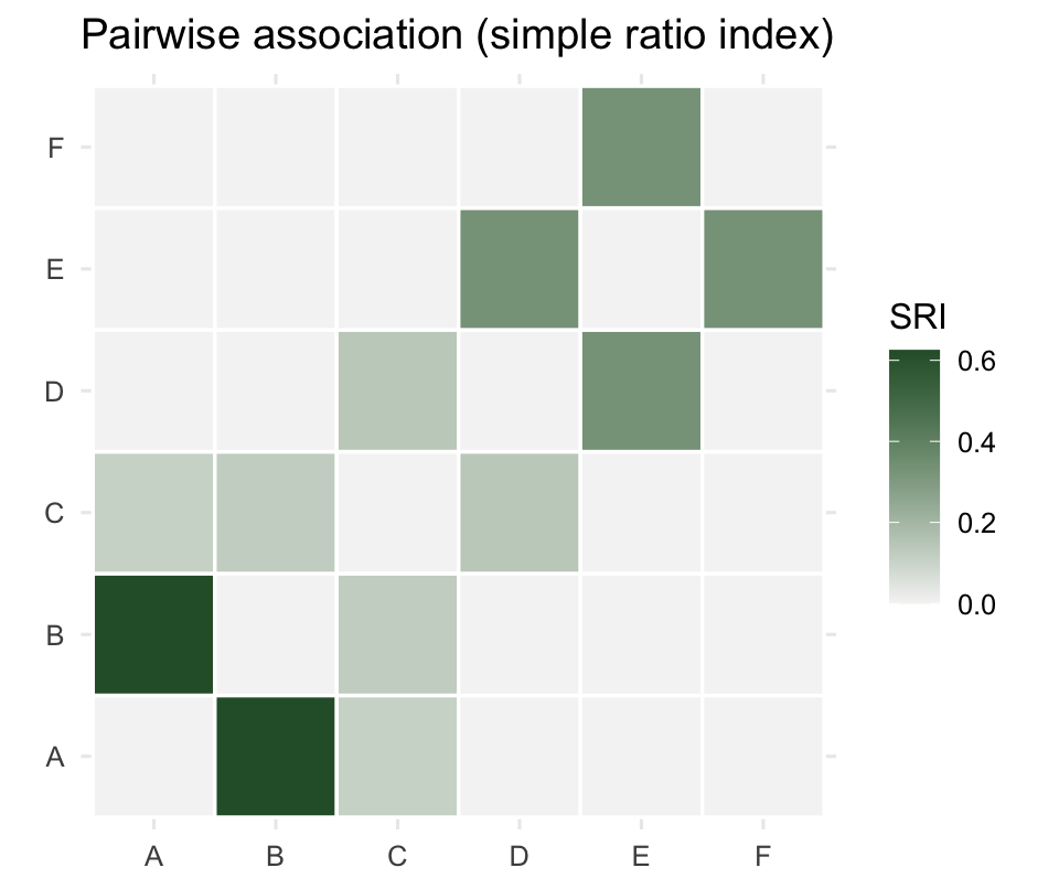
Read the table top to bottom. A and B were together five times ($x = 5$) and never seen singly enough to pull them apart, giving SRI `r round(sri["A","B"],3)` and HWI `r round(hwi["A","B"],3)`. Down among the weaker pairs, D and E sit together only twice against four periods in which just one of them was recorded, so the two indices split further apart. The C to D edge is a single shared group: a thin bridge between what look like two clusters.
The association matrix makes the clusters visible.
```{r}
#| label: fig-heatmap
#| fig-cap: "Simple ratio index for every pair. A and B stand out; D to F holds together through E, and a single weak C to D cell is all that links the two groups."
#| fig-alt: "A six by six heatmap of association indices with the same six animals on both axes, A at the lower left and F at the upper right. One cell is much darker than the rest, A with B. D with E and E with F are mid green, D with F is the palest tint, and the A to C and B to C cells are barely tinted. A faint C to D cell is the only link between the two groups, and the diagonal sits at the palest tint as well."
#| fig-width: 5
#| fig-height: 4.2
long <- expand.grid(i = ids, j = ids)
long$sri <- mapply(function(a, b) sri[a, b], long$i, long$j)
ggplot(long, aes(i, j, fill = sri)) +
  geom_tile(colour = "#cfcdc0", linewidth = 0.6) +
  scale_fill_gradient(low = "#e6e4d8", high = "#2b5d34", name = "SRI") +
  coord_equal() +
  labs(x = NULL, y = NULL,
       title = "Pairwise association (simple ratio index)")
```
## Where the choice bites
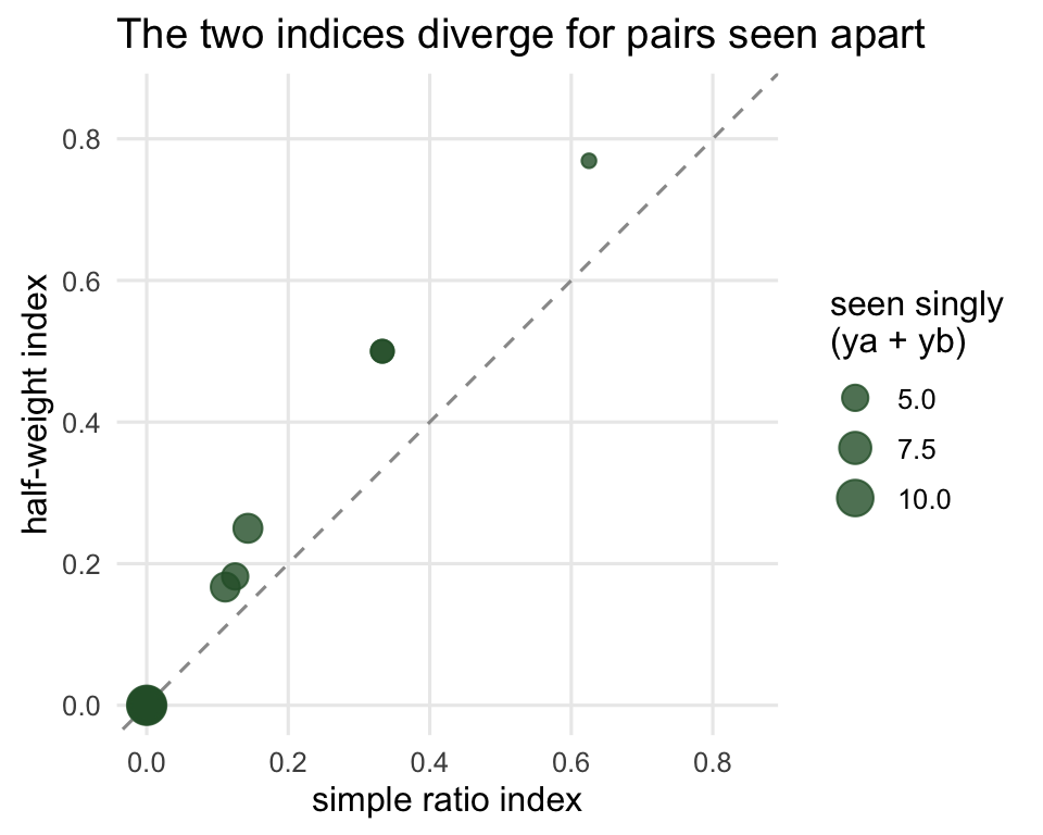
For the tight pairs the two indices tell the same story; the ranking of edges barely moves. The gap is widest for pairs whose single sightings are comparable in number to their joint ones, and that gap is not tiny.
```{r}
#| label: fig-divergence
#| fig-cap: "Half-weight against simple ratio for every pair. Points on the dashed line would mean the indices agree; the pairs whose single sightings are comparable in number to their joint ones sit furthest above it, and those seen together only rarely sit closer to it. Pairs never seen together sit at the origin, however often they were seen apart."
#| fig-alt: "A scatter plot with the simple ratio index on the x axis and the half-weight index on the y axis, both from zero to about 0.85. A dashed identity line runs diagonally. Points lie on or above the line, with a cluster of large points at the origin and the largest vertical gaps at middling association values."
#| fig-width: 5
#| fig-height: 4
ggplot(tab, aes(SRI, HWI)) +
  geom_abline(slope = 1, intercept = 0, linetype = "dashed", colour = "grey60") +
  geom_point(aes(size = ya + yb), colour = "#2b5d34", alpha = 0.8) +
  scale_size_continuous(name = "seen singly\n(ya + yb)", range = c(2, 6)) +
  coord_equal(xlim = c(0, 0.85), ylim = c(0, 0.85)) +
  labs(title = "The gap is widest at middling association",
       x = "simple ratio index", y = "half-weight index")
```
```{r}
#| label: maxgap
c(max_HWI_minus_SRI = round(max(abs(tab$diff)), 3),
  edges_present = sum(sri[upper.tri(sri)] > 0),
  dyads_total = n * (n - 1) / 2)
```
The largest gap between the indices for this dataset is `r round(max(abs(tab$diff)),3)`, and it lands on D to E and E to F: two together-sightings each against four single ones. It is the ratio that drives the divergence, not the raw count of single sightings. The pairs seen apart most often here are the ones never seen together at all, and both indices score those zero. On this dataset that gap reorders nothing: both indices put the six non-zero edges in the same order. What a gap of that size can change is a threshold decision, since on a scale from zero to one it will move a pair above or below whatever cut you later use to draw the network. The indices agree on the order and disagree on the values, and the disagreement peaks at middling association strengths, which is precisely the range where marginal associations get decided.
## What this settles and what it does not
The practical rule is short. Use the simple ratio index when you are confident that seeing one animal without its partner really means they were apart, so the single-identification counts are trustworthy. Reach for the half-weight index when your protocol tends to miss the second animal of a pair, so those counts are inflated. Whichever you choose, report it: an SRI network and an HWI network from the same sightings are not interchangeable at the edges.
Two limits are worth stating now. First, both indices rest on the gambit of the group, and a weight of `r round(sri["A","B"],3)` between A and B means "seen in the same group five times out of eight", not "socially bonded". Second, the whole thing depends on how a group was defined in the field, and that definition is a decision you made, not a fact the animals handed you. The checking post takes both of these apart.
With the network in hand, the next question is whether any of its structure is real or whether it is what random mixing would produce anyway. That needs a null model, and for social networks the choice of null is the difference between a sound result and a confident mistake.
## Where to go next
Build the network first, then interrogate it. The permutation post shows how to ask whether the associations you measured are more than chance, and why the obvious shuffle gives the wrong answer. The centrality post turns the matrix into per-individual scores, and the checking post returns to the two assumptions flagged above.
## References
Cairns SJ, Schwager SJ 1987 Animal Behaviour 35(5):1454-1469 (10.1016/S0003-3472(87)80018-0)
Whitehead H 2008 Analyzing Animal Societies: Quantitative Methods for Vertebrate Social Analysis. University of Chicago Press. ISBN 978-0226895215
Farine DR, Whitehead H 2015 Journal of Animal Ecology 84(5):1144-1163 (10.1111/1365-2656.12418)
## Related tutorials
- [Permutation tests for social networks](../permutation-tests-social-networks/)
- [Network centrality and sampling effort](../network-centrality-sampling-effort/)
- [Checking a social network analysis](../checking-a-social-network-analysis/)
- [Co-occurrence null models](../co-occurrence-null-models/)