---
title: "Network centrality and sampling effort"
description: "Degree, strength and eigenvector centrality for an animal social network in R: each measures something different, and all three rise with sighting effort."
date: "2026-06-19 13:00"
date-modified: "2026-10-07"
categories: [R, social networks, network centrality, animal behaviour, ecology tutorial]
image: thumbnail.png
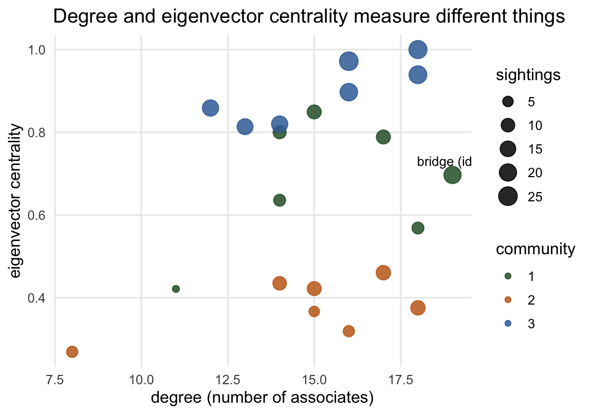
image-alt: "A scatter of eigenvector centrality against degree, with one labelled bridging individual at the highest degree but an eigenvector score near 0.7, below the top nodes close to 1.0."
---
*Corrected 7 October 2026: the post said that the individuals seen most have the highest strength; strength only tends to rise with the sighting count, not in strict order, and the sentence now says so.*
You have a weighted social network and you want a number per individual: who is central, who is peripheral, who holds the group together. That number is a centrality metric, and there are several. This post computes three of them by hand, shows that they disagree because they measure different things, and then delivers the caveat that undoes a lot of published rankings: raw centrality climbs with how often you saw the animal.
```{r}
#| label: setup
#| code-fold: true
#| code-summary: "Setup: packages, colours and plot theme"
#| results: hide
#| message: false
#| warning: false
library(ggplot2)
theme_set(theme_minimal(base_size = 12) +
  theme(plot.background = element_rect(fill = "#f5f4ee", colour = NA),
        panel.background = element_rect(fill = "#f5f4ee", colour = NA),
        panel.grid.minor = element_blank()))
knitr::opts_chunk$set(dev.args = list(bg = "#f5f4ee"))
```
## Three notions of central
Start from the association matrix, the simple ratio index network built in [association indices for social networks](../association-indices-social-networks/). Three metrics fall straight out of it.
- **Degree** counts an individual's distinct associates: how many others it has a non-zero edge to. It ignores edge weight.
- **Strength** sums the edge weights: total association across all partners. A few strong bonds and many weak ones can give the same strength.
- **Eigenvector centrality** rewards being connected to individuals who are themselves well connected. It is the leading eigenvector of the matrix, so an individual scores highly by sitting inside a dense, well-linked cluster, not merely by having many edges.
Here they are, each a one-liner.
```{r}
#| label: metrics
sri_from_gbi <- function(gbi) {
  co <- crossprod(gbi); n <- diag(co)
  a <- co / (outer(n, n, "+") - co); diag(a) <- 0; a
}
node_degree   <- function(a) rowSums(a > 0)
node_strength <- function(a) rowSums(a)
eigen_cent    <- function(a) { e <- eigen(a, symmetric = TRUE); v <- abs(e$vectors[, 1]); v / max(v) }
```
Now a population to try them on: three communities of differing cohesion, sighting effort that varies mildly across individuals, and one animal (number seven) that lives in the first community but also joins the second, a bridge between them.
```{r}
#| label: population
set.seed(4)
n_ind <- 21; n_grp <- 55
community <- rep(1:3, each = 7)
effort <- runif(n_ind, 0.85, 1.3)
cohesion <- c(0.70, 0.40, 0.55)[community]
bridge <- 7
gbi <- matrix(0L, n_grp, n_ind)
for (k in 1:n_grp) {
  fc <- sample(1:3, 1)
  base <- ifelse(community == fc, cohesion, 0.05) * effort
  if (fc == 2) base[bridge] <- 0.45
  gbi[k, ] <- rbinom(n_ind, 1, pmin(base, 0.95))
}
gbi <- gbi[rowSums(gbi) > 0, ]; keep <- colSums(gbi) > 0; gbi <- gbi[, keep]
community <- community[keep]; count <- colSums(gbi)

net <- sri_from_gbi(gbi)
deg <- node_degree(net); str <- node_strength(net); eig <- eigen_cent(net)
```
## They do not agree
If the three metrics ranked individuals the same way, you would only ever need one. They do not.
```{r}
#| label: rank-cor
c(degree_vs_strength = round(cor(deg, str, method = "spearman"), 3),
  degree_vs_eigen    = round(cor(deg, eig, method = "spearman"), 3),
  strength_vs_eigen  = round(cor(str, eig, method = "spearman"), 3))
```
Strength and eigenvector centrality track each other fairly closely. Degree parts company with both: its rank correlation with eigenvector centrality is only about 0.21. Degree and eigenvector centrality are answering different questions, and on this network the answers barely line up.
The bridging individual is where the disagreement becomes a story.
```{r}
#| label: ranks
ranks <- data.frame(
  id = seq_len(ncol(gbi)), community = community, count = count,
  degree_rank = rank(-deg), strength_rank = rank(-str), eigen_rank = rank(-eig))
ranks[order(ranks$strength_rank), ][1:6, ]
```
Individual twenty tops both strength and eigenvector centrality: a well-embedded member of a cohesive community, connected to others who are themselves connected. Individual seven, the bridge, is a different animal. It has the highest degree in the network (it associates with the most distinct others, because it moves between two communities) yet its eigenvector centrality is only middling: its partners are split across two groups rather than concentrated in one dense core, so it does not sit at the heart of any single cluster. Degree calls it the most central animal in the population; eigenvector centrality calls it ordinary. Both are right about their own question.
```{r}
#| label: fig-disagree
#| fig-cap: "Eigenvector centrality against degree, one point per individual, coloured by community. The relationship is weak, and the bridging individual (labelled) sits below the most embedded individuals: many associates, but only a middling eigenvector score."
#| fig-alt: "A scatter plot of eigenvector centrality on the y axis against degree on the x axis, with points coloured by one of three communities. The points are loosely scattered rather than lying on a line. One point at high degree but low-to-middling eigenvector centrality is labelled as the bridge individual, sitting below the most embedded individuals rather than at the top of the cloud."
#| fig-width: 6
#| fig-height: 4.2
df <- data.frame(id = seq_len(ncol(gbi)), degree = deg, eigen = eig,
                 community = factor(community), count = count)
ggplot(df, aes(degree, eigen, colour = community)) +
  geom_point(aes(size = count), alpha = 0.85) +
  annotate("text", x = df$degree[bridge], y = df$eigen[bridge],
           label = "bridge (id 7)", vjust = -1, hjust = 1, size = 3.4) +
  scale_colour_manual(values = c("#2b5d34", "#c46a1b", "#3a6ea5")) +
  scale_size_continuous(name = "sightings", range = c(2, 6)) +
  labs(title = "Degree and eigenvector centrality measure different things",
       x = "degree (number of associates)", y = "eigenvector centrality")
```
## The number that spoils the ranking
Now the caveat. Pick any of these metrics and correlate it with how many times each individual was seen.
```{r}
#| label: effort-confound
c(cor_strength_count = round(cor(str, count), 3),
  count_range_low  = min(count),
  count_range_high = max(count))
```
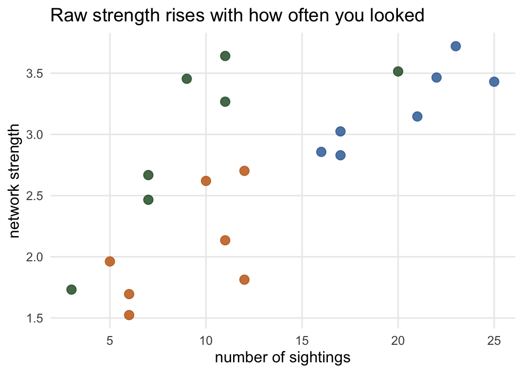
Strength correlates with sighting count at about 0.72. Individuals here were seen between three and twenty-five times, and strength tends to rise with the count, though not in strict order. Some of that is real (a genuinely gregarious animal turns up more and associates more), but some of it is pure sampling: watch an animal more and its measured associations accumulate, whatever its true sociality. Degree and eigenvector centrality carry the same passenger. A centrality ranking, taken at face value, can be a ranking of who your field protocol happened to record most.
```{r}
#| label: fig-effort
#| fig-cap: "Strength against sighting count. The upward trend means part of what the ranking calls sociality is really observation effort."
#| fig-alt: "A scatter plot of network strength on the y axis against the number of sightings on the x axis, with points coloured by community. The points rise from lower left to upper right, showing a clear positive relationship between how often an individual was seen and its network strength."
#| fig-width: 5.6
#| fig-height: 4
df$strength <- str
ggplot(df, aes(count, strength, colour = community)) +
  geom_point(size = 3, alpha = 0.85) +
  scale_colour_manual(values = c("#2b5d34", "#c46a1b", "#3a6ea5"), guide = "none") +
  labs(title = "Raw strength rises with how often you looked",
       x = "number of sightings", y = "network strength")
```
## What to do about it
Do not read a raw centrality ranking as a sociality ranking until you have looked at this scatter. Two honest routes forward. You can control for effort directly: regress the metric on sighting count and work with the residual, the part of centrality that is not explained by how often the animal was seen. That route has a price the sentence hides: the residual is an estimate, not a measurement, and a second analysis that treats it as data misstates its own uncertainty, spending power when the effort slope was fitted on these same animals and understating the interval when the slope was borrowed from elsewhere, which [residuals as a variable](../residuals-as-a-variable/) measures. Or you can test centrality against the data-stream null from the permutation post, which rebuilds the network under random association with the same sighting counts, so the effort component sits in the null instead of in your result. Both say the same thing in different dialects: separate the sociality from the sampling before you rank anyone.
Which metric you report should follow your question, not habit. Degree for reach, how many others an individual contacts. Strength for total association. Eigenvector centrality for being embedded among the well connected. They are not substitutes, and the bridge above is the proof: it is the most central animal or an unremarkable one depending only on which you pick.
## Where to go next
The checking post makes this effort diagnostic step one of a short routine, then adds two more: whether your data even has the power to detect real structure, and whether the group definition underneath the whole network holds up. The permutation post is where the data-stream null comes from, and the association-index post covers how the edge weights were built in the first place.
## References
Farine DR, Whitehead H 2015 Journal of Animal Ecology 84(5):1144-1163 (10.1111/1365-2656.12418)
Whitehead H 2008 Analyzing Animal Societies: Quantitative Methods for Vertebrate Social Analysis. University of Chicago Press. ISBN 978-0226895215
Croft DP, James R, Krause J 2008 Exploring Animal Social Networks. Princeton University Press. ISBN 978-0691127521
## Related tutorials
- [Association indices for social networks](../association-indices-social-networks/)
- [Permutation tests for social networks](../permutation-tests-social-networks/)
- [Checking a social network analysis](../checking-a-social-network-analysis/)
- [Dominance hierarchies from wins](../dominance-hierarchies-from-wins/)