library(ggplot2)
library(patchwork)

te_paper  <- "#f5f4ee"
te_ink    <- "#16241d"
te_body   <- "#2c3a31"
te_forest <- "#275139"
te_rust   <- "#b5534e"
te_gold   <- "#c9b458"
te_line   <- "#dad9ca"

theme_datasheet <- function() {
  theme_minimal(base_size = 12) +
    theme(plot.background  = element_rect(fill = te_paper, colour = NA),
          panel.background = element_rect(fill = te_paper, colour = NA),
          panel.grid.major = element_line(colour = te_line, linewidth = 0.3),
          panel.grid.minor = element_blank(),
          text             = element_text(colour = te_body),
          plot.title       = element_text(colour = te_ink, face = "bold"),
          plot.subtitle    = element_text(colour = te_body),
          axis.text        = element_text(colour = te_body))
}

n_ind   <- 10
ids     <- LETTERS[seq_len(n_ind)]
ability <- setNames(seq(2.4, -2.4, length.out = n_ind), ids)
n_many  <- 20
n_few   <- 1

encounters <- matrix(n_few, n_ind, n_ind, dimnames = list(ids, ids))
diag(encounters) <- 0
encounters["G", c("H", "I", "J")] <- n_many
encounters[c("H", "I", "J"), "G"] <- n_many
encounters["A", c("B", "C", "D")] <- n_many
encounters[c("B", "C", "D"), "A"] <- n_many

simulate_wins <- function(seed) {
  set.seed(seed)
  W <- matrix(0, n_ind, n_ind, dimnames = list(ids, ids))
  for (i in seq_len(n_ind - 1)) for (j in (i + 1):n_ind) {
    k <- encounters[i, j]
    if (k == 0) next
    p <- 1 / (1 + exp(-(ability[i] - ability[j])))
    w <- rbinom(1, k, p)
    W[i, j] <- w
    W[j, i] <- k - w
  }
  W
}
wins  <- simulate_wins(31)
total <- wins + t(wins)Dominance hierarchies from wins
R
behaviour
social structure
statistics
ecology tutorial
Proportion of wins ranks who an animal fought, not how good it is. David’s score, Bradley-Terry and Elo compared on a win matrix in base R, no packages.
Watch a group for a season, write down who displaced whom, and you have a square matrix of wins. Turning that into an order looks like counting: whoever wins the highest share of their contests goes on top.
That works when everybody fights everybody equally often, and no group does. Some pairs meet constantly and some almost never, and an animal’s win rate is then a statement about who it happened to face as much as about what it can do. The corrections for this are old, they are short, and none of the standard ones needs a package.
This post builds a group where the answer is known, shows the proportion of wins putting a middling animal on top, and works through what David’s score, Bradley-Terry and Elo each do about it. All four are written out in base R, which is also the only way to see what each one is weighting.
A group with a known order
Ten animals with abilities on a logistic scale, and an encounter design of the sort field data actually has: two animals contest a lot with a few specific partners and once with everybody else.
A is the strongest animal and J the weakest. G sits seventh of ten, and G’s contests are almost all against the three animals below it. A’s are almost all against the three animals just below it, which are the hardest opponents in the group after A itself.
prop_win  <- rowSums(wins) / rowSums(total)
mean_opp  <- as.numeric(total %*% ability) / rowSums(total)
names(mean_opp) <- ids
n_events  <- sum(wins)
opp_gap   <- mean_opp["A"] - mean_opp["G"]
159 recorded contests. The average opponent A faced has an ability of +1.12 and the average opponent G faced has -1.60, a gap of 2.72 on the same scale the abilities are measured on.
The proportion of wins ranks the opponents
rank_of  <- function(x) rank(-x, ties.method = "min")
prop_top <- names(which.max(prop_win))
prop_rho <- cor(prop_win, ability, method = "spearman")
g_rank_p <- rank_of(prop_win)["G"]
G wins 74.2 per cent of its contests and A wins 71.2 per cent, so the win rate ranks G first, above A. G is seventh of ten. The Spearman correlation between the win rate and the true ability is 0.63, which is not nothing, and is also not an ordering anyone should report.
The mechanism is not observation effort. Effort inflates centrality scores in association networks, which is a separate problem covered elsewhere on the site, and it would show up here as a confounding between win rate and number of contests. What is happening instead is that a win rate has no way to express that one animal’s wins were harder to get than another’s.
Two corrections, and what each one weights
David’s score replaces the raw count with a sum of dyadic proportions, then adds a second round weighted by how strong each defeated opponent was, and subtracts the same construction for losses.
dyadic <- function(W, corrected) {
  tt <- W + t(W)
  P  <- ifelse(tt > 0, W / pmax(tt, 1), 0)
  if (corrected) P <- ifelse(tt > 0, P - (P - 0.5) / (tt + 1), 0)
  P
}
david_score <- function(W, corrected = FALSE) {
  P  <- dyadic(W, corrected)
  w1 <- rowSums(P)
  l1 <- colSums(P)
  setNames(w1 + as.numeric(P %*% w1) - l1 - as.numeric(t(P) %*% l1), ids)
}
ds_raw  <- david_score(wins)
ds_corr <- david_score(wins, corrected = TRUE)
Bradley-Terry goes further and writes a likelihood. Each animal gets a latent ability, the probability that i beats j is the logistic function of the difference, and the whole thing is an ordinary binomial regression on a design matrix of plus and minus ones.
bt_design <- function(W) {
  tt <- W + t(W)
  pr <- which(upper.tri(tt) & tt > 0, arr.ind = TRUE)
  X  <- matrix(0, nrow(pr), n_ind, dimnames = list(NULL, ids))
  for (r in seq_len(nrow(pr))) {
    X[r, pr[r, 1]] <-  1
    X[r, pr[r, 2]] <- -1
  }
  list(X = X[, -n_ind, drop = FALSE],
       y = cbind(W[cbind(pr[, 1], pr[, 2])], W[cbind(pr[, 2], pr[, 1])]))
}
bt_fit <- function(W) {
  d <- bt_design(W)
  suppressWarnings(glm(d$y ~ 0 + d$X, family = binomial))
}
bt_ability <- function(W) {
  a <- c(coef(bt_fit(W)), 0)
  names(a) <- ids
  a - mean(a)
}
bt_hat  <- bt_ability(wins)
bt_rho  <- cor(bt_hat, ability, method = "spearman")
dsr_rho <- cor(ds_raw, ability, method = "spearman")
dsc_rho <- cor(ds_corr, ability, method = "spearman")
g_rank_dsr <- rank_of(ds_raw)["G"]
g_rank_bt  <- rank_of(bt_hat)["G"]
bt_top     <- names(which.max(bt_hat))
bt_misplaced <- sum(rank_of(bt_hat) != rank_of(ability))
Both corrections put G back where it belongs. David’s score moves it from first to 7, Bradley-Terry to 7, and the Bradley-Terry ordering here misplaces only 2 animals, the weakest pair, adjacent in the true order, which swap places, with A on top and a Spearman of 0.99.
rank_tab <- data.frame(
  id    = rep(ids, 4),
  truth = rep(rank_of(ability), 4),
  est   = c(rank_of(prop_win), rank_of(ds_raw), rank_of(ds_corr), rank_of(bt_hat)),
  score = rep(c("proportion of wins", "David's score",
                "David's score, corrected", "Bradley-Terry"), each = n_ind))
rank_tab$score <- factor(rank_tab$score,
  levels = c("proportion of wins", "David's score",
             "David's score, corrected", "Bradley-Terry"))

rank_tab$focal <- ifelse(rank_tab$id == "G", "G", "the rest")

ggplot(rank_tab, aes(truth, est, colour = focal)) +
  geom_abline(slope = 1, intercept = 0, colour = te_line, linewidth = 0.8) +
  geom_point(size = 2.8) +
  scale_colour_manual(values = c(te_rust, te_forest), name = NULL) +
  scale_x_continuous(breaks = seq(1, n_ind, 3)) +
  scale_y_continuous(breaks = seq(1, n_ind, 3)) +
  facet_wrap(~score, nrow = 1) +
  labs(x = "true rank", y = "estimated rank",
       title = "One animal in the wrong place, and where each score puts it") +
  theme_datasheet() +
  theme(legend.position = "bottom",
        strip.text = element_text(colour = te_ink, face = "bold", size = 9))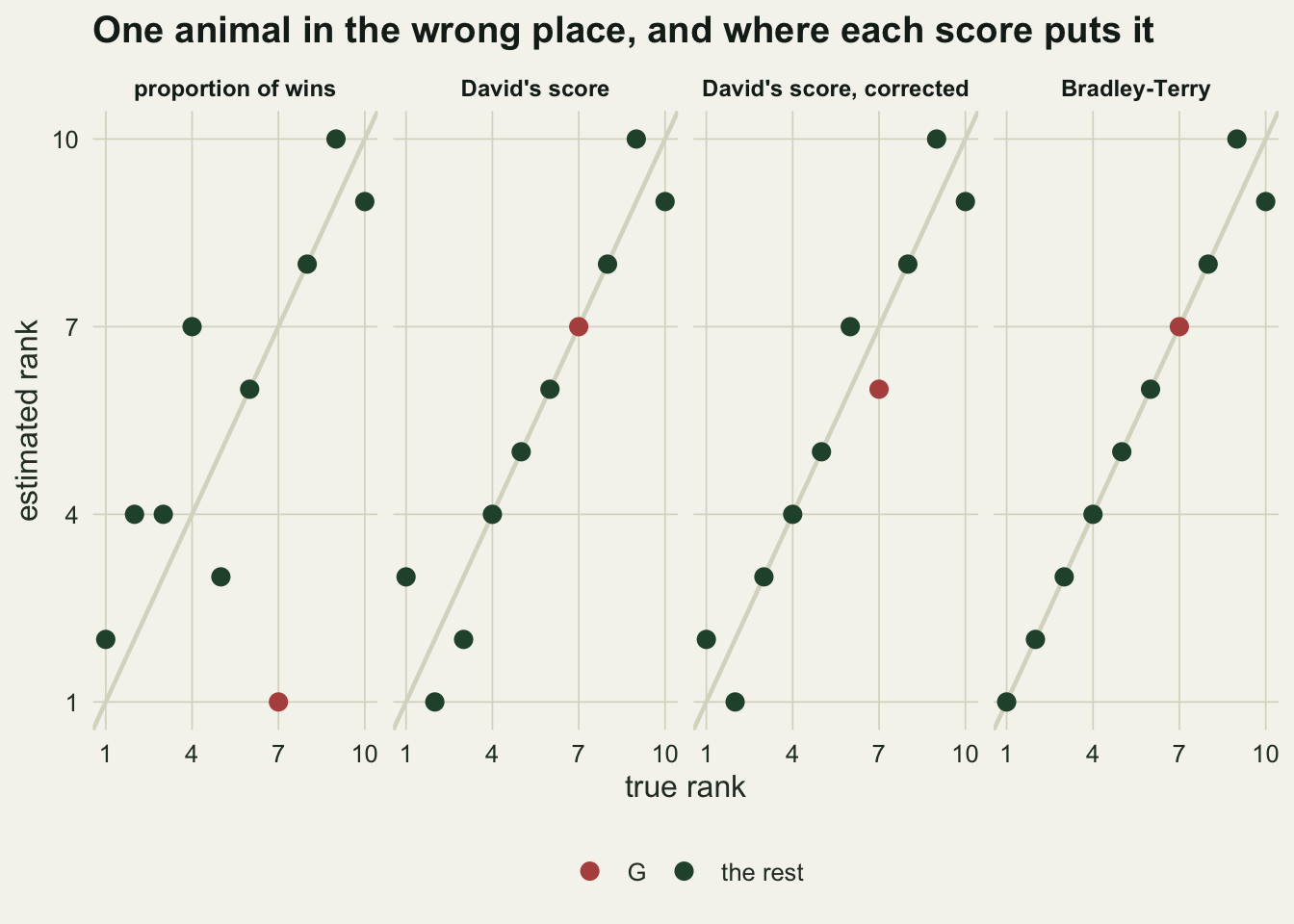
One group is an anecdote, so here is the same design simulated three hundred times.
n_set  <- 300
sweep_scores <- t(vapply(seq_len(n_set), function(s) {
  W  <- simulate_wins(s)
  tt <- W + t(W)
  pw <- rowSums(W) / rowSums(tt)
  dr <- david_score(W)
  dc <- david_score(W, corrected = TRUE)
  bh <- bt_ability(W)
  c(cor(pw, ability, method = "spearman"), cor(dr, ability, method = "spearman"),
    cor(dc, ability, method = "spearman"), cor(bh, ability, method = "spearman"),
    rank_of(pw)["G"], rank_of(dr)["G"], rank_of(dc)["G"], rank_of(bh)["G"],
    names(which.max(pw)) != "A", names(which.max(dr)) != "A",
    names(which.max(dc)) != "A", names(which.max(bh)) != "A")
}, numeric(12)))
score_names <- c("proportion of wins", "David's score",
                 "David's score, corrected", "Bradley-Terry")
summ <- data.frame(
  score    = factor(score_names, levels = score_names),
  rho      = colMeans(sweep_scores[, 1:4]),
  g_rank   = colMeans(sweep_scores[, 5:8]),
  top_miss = colMeans(sweep_scores[, 9:12]),
  g_top3   = colMeans(sweep_scores[, 5:8] <= 3))
top3_cut  <- 3
g_top3_max <- max(summ$g_top3[2:4])
g_rank_mid <- mean(summ$g_rank[2:4])
mc_half    <- 0.5
The win rate places the seventh ranked animal in the top 3 in 98 per cent of the simulated groups, with a mean rank of 2.0. Both versions of David’s score and Bradley-Terry put it in the top 3 in at most 1.7 per cent, with mean ranks around 6.5. On the whole ordering the mean Spearman rises from 0.60 to 0.92 and 0.95.
The error at the top is the more interesting number. Asked only who the top animal is, the raw David’s score is wrong 41 per cent of the time, which is worse than the win rate at 20 per cent. The chance corrected version drops to 15 per cent and Bradley-Terry to 12 per cent.
rho_long <- data.frame(
  rho   = as.numeric(sweep_scores[, 1:4]),
  score = factor(rep(score_names, each = n_set), levels = score_names))

p_rho <- ggplot(rho_long, aes(score, rho, fill = score)) +
  geom_boxplot(outlier.size = 0.6, colour = te_ink, linewidth = 0.35) +
  scale_fill_manual(values = c(te_rust, te_gold, te_ink, te_forest)) +
  labs(x = NULL, y = "Spearman with true ability",
       title = "Whole ordering") +
  theme_datasheet() +
  theme(legend.position = "none",
        axis.text.x = element_text(angle = 25, hjust = 1, size = 9))

p_top <- ggplot(summ, aes(score, 100 * top_miss, fill = score)) +
  geom_col(width = 0.65) +
  scale_fill_manual(values = c(te_rust, te_gold, te_ink, te_forest)) +
  labs(x = NULL, y = "per cent of groups", title = "Wrong animal named first") +
  theme_datasheet() +
  theme(legend.position = "none",
        axis.text.x = element_text(angle = 25, hjust = 1, size = 9))

p_rho + p_top + plot_annotation(theme = theme_datasheet())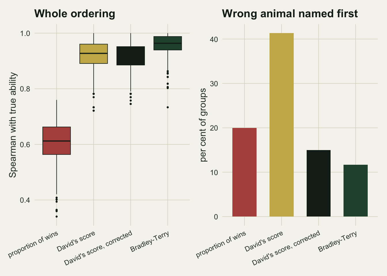
The reason is visible in the code. David’s score builds from a matrix of dyadic proportions, and a dyad seen once contributes a proportion of zero or one exactly as firmly as a dyad seen twenty times. In this design most dyads were seen once, so most of the score is carried by the least informative cells. Bradley-Terry never forms a proportion: it counts wins and losses in a likelihood, so a dyad contributes in proportion to how often it was contested. The chance corrected dyadic index, which pulls a proportion towards one half by an amount that depends on the number of encounters, closes most of the gap for the price of one extra term.
When the likelihood has no answer
Bradley-Terry has one structural requirement, and glm() will not tell you when it fails. The maximum likelihood estimate exists only if the digraph of wins is strongly connected: for every way of splitting the group into two parts, somebody in each part must have beaten somebody in the other. Otherwise one group of animals can be pushed arbitrarily far above the other and the likelihood keeps improving.
mat_pow <- function(A, k) {
  B <- diag(nrow(A))
  for (i in seq_len(k)) B <- B %*% A
  B
}
strongly_connected <- function(W) all(mat_pow((W > 0) + diag(nrow(W)), nrow(W) - 1) > 0)

conn <- t(vapply(seq_len(n_set), function(s) {
  W <- simulate_wins(s)
  m <- bt_fit(W)
  c(strongly_connected(W),
    any(rowSums(W) == 0) || any(colSums(W) == 0),
    max(abs(coef(m))))
}, numeric(3)))

share_broken  <- mean(conn[, 1] == 0)
share_extreme <- mean(conn[, 2] == 1)
big_coef      <- median(conn[conn[, 1] == 0, 3])
ok_coef       <- median(conn[conn[, 1] == 1, 3])
Across the three hundred groups the digraph fails to be strongly connected in 17 per cent of them, while an animal that never won or never lost turns up in only 1.3 per cent. Scanning for an undefeated alpha or a hopeless omega therefore catches almost none of the cases, which is the argument for running the digraph test instead. In the affected groups the largest fitted ability has a median absolute value of 24 against 5.3 in the rest, and the standard errors go with them.
undefeated <- wins
undefeated["A", ] <- undefeated["A", ] + undefeated[, "A"]
undefeated[, "A"] <- 0
diag(undefeated) <- 0

m_sep  <- bt_fit(undefeated)
se_sep <- max(summary(m_sep)$coefficients[, 2])
ab_sep <- max(abs(coef(m_sep)))
conn_sep <- strongly_connected(undefeated)

half_add <- undefeated
seen     <- (undefeated + t(undefeated)) > 0
half_add[seen] <- half_add[seen] + 0.5
m_half  <- bt_fit(half_add)
se_half <- max(summary(m_half)$coefficients[, 2])
a_half  <- c(coef(m_half), 0); names(a_half) <- ids
a_half  <- a_half - mean(a_half)
Handing A every one of its contests makes the point loudly. The digraph test returns FALSE, glm() returns coefficients as large as 108 with standard errors up to 37698, and it does so after converging without an error. Adding half a win to each side of every observed dyad brings the largest standard error down to 0.69 and A’s ability to 2.90, at the cost of shrinking every other estimate as well. A penalty or a weakly informative prior is the same repair with a better justification, and the site covers what that looks like for logistic regression in general.
Elo depends on the order you feed it
Elo updates a rating after every contest, which makes it attractive for long observation records and gives it a property the other two do not have: the answer depends on the sequence.
elo_run <- function(seq_i, seq_j, k_factor, init_rating = 1000) {
  r <- setNames(rep(init_rating, n_ind), ids)
  for (t in seq_along(seq_i)) {
    i <- seq_i[t]; j <- seq_j[t]
    p <- 1 / (1 + 10^((r[j] - r[i]) / 400))
    r[i] <- r[i] + k_factor * (1 - p)
    r[j] <- r[j] - k_factor * (1 - p)
  }
  r
}

event_i <- rep(row(wins)[wins > 0], wins[wins > 0])
event_j <- rep(col(wins)[wins > 0], wins[wins > 0])

n_shuffle <- 500
k_grid    <- c(20, 50, 100, 200)
set.seed(4)
elo_sweep <- do.call(rbind, lapply(k_grid, function(kk) {
  out <- t(replicate(n_shuffle, {
    o <- sample(length(event_i))
    r <- elo_run(event_i[o], event_j[o], kk)
    c(cor(r, ability, method = "spearman"), which.max(r), r["A"] - r["B"])
  }))
  data.frame(k_factor = kk, rho = out[, 1],
             top_miss = out[, 2] != 1, gap = out[, 3])
}))
elo_summ <- aggregate(cbind(rho, top_miss, gap) ~ k_factor, elo_sweep, mean)
elo_sd   <- aggregate(cbind(rho, gap) ~ k_factor, elo_sweep, sd)
elo_neg  <- aggregate(gap ~ k_factor, elo_sweep, function(v) mean(v < 0))
k_mid    <- 100
row_mid  <- which(elo_summ$k_factor == k_mid)
The contests are the same contests in every one of the 500 runs; only the order changes. At an update constant of 100 the mean Spearman with the truth is 0.90, which is respectable, and the animal with the highest final rating is not A in 34 per cent of orderings. The rating gap between A and B averages 87 points with a standard deviation of 120, and it comes out negative on 24 per cent of the orderings.
p_k1 <- ggplot(elo_summ, aes(k_factor, rho)) +
  geom_line(colour = te_forest, linewidth = 0.9) +
  geom_point(colour = te_forest, size = 2.6) +
  labs(x = NULL, y = "mean Spearman", title = "A larger update learns faster") +
  theme_datasheet()

p_k2 <- ggplot(elo_summ, aes(k_factor, 100 * top_miss)) +
  geom_line(colour = te_rust, linewidth = 0.9) +
  geom_point(colour = te_rust, size = 2.6) +
  labs(x = "update constant", y = "per cent of orderings",
       title = "And forgets the past faster") +
  theme_datasheet()

p_k1 / p_k2 + plot_annotation(theme = theme_datasheet())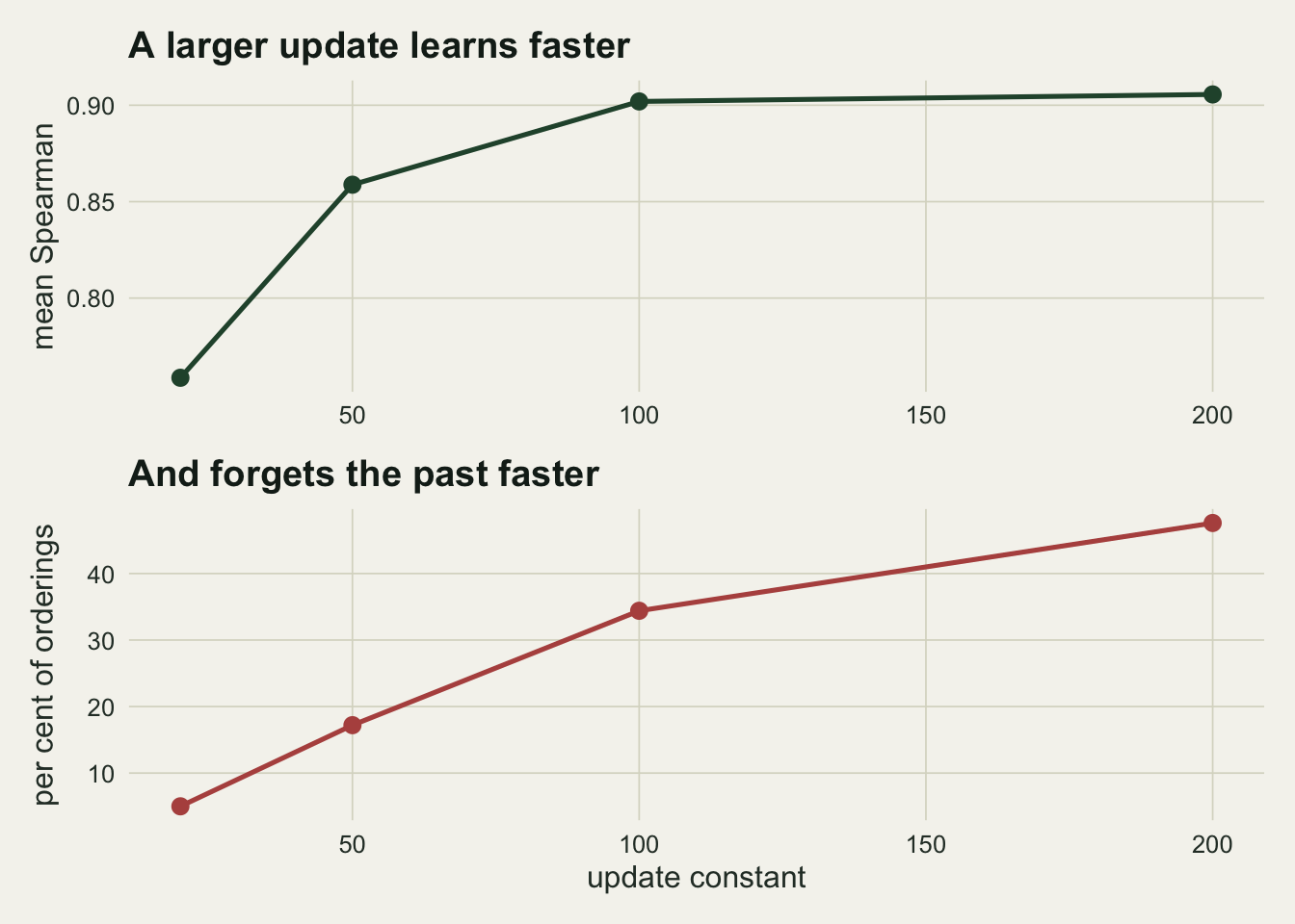
Raising the update constant helps the ordering, because the ratings reach a sensible spread within a short record, and hurts the top of it, because the last few contests then carry most of the weight. There is no setting that removes the dependence, only settings that trade one symptom for the other. If the ratings are meant to describe a stable hierarchy rather than track a changing one, that dependence is pure noise, and the only honest use of a single Elo ordering is one that reports how much it moves under reordering.
Is the order linear, and against what
A hierarchy is linear when the animals can be written in a single order that every contest respects. Landau’s h is the standard measure of how close a win matrix comes to that. Give each animal a score V, the number of distinct opponents it beat, and h is the spread of those scores divided by the spread a perfect order would produce.
landau_V <- function(W, unknown = 0) {
  tt <- W + t(W)
  D  <- ifelse(tt == 0, unknown, ifelse(W > t(W), 1, ifelse(W < t(W), 0, 0.5)))
  diag(D) <- 0
  rowSums(D)
}
landau_h <- function(W, unknown = 0) {
  N <- nrow(W)
  12 / (N^3 - N) * sum((landau_V(W, unknown) - (N - 1) / 2)^2)
}
h_obs   <- landau_h(wins)
V_obs   <- landau_V(wins)
h_line  <- landau_h(matrix(upper.tri(diag(n_ind)) * 1, n_ind, n_ind))
cyc3    <- matrix(0, 3, 3); cyc3[cbind(c(1, 2, 3), c(2, 3, 1))] <- 1
h_cycle <- landau_h(cyc3)

n_dyad <- n_ind * (n_ind - 1) / 2
ij_all <- which(upper.tri(matrix(0, n_ind, n_ind)), arr.ind = TRUE)

circ_triads <- function(W) choose(nrow(W), 3) - sum(choose(landau_V(W), 2))
d_obs   <- circ_triads(wins)
d_all   <- choose(n_ind, 3)
h_via_d <- 1 - 24 * d_obs / (n_ind^3 - n_ind)
d_null  <- d_all / 4

h_ceiling <- 3 * (n_ind - 1) / (n_ind + 1)
h_fixed_cut <- 0.9                        # the cut the literature uses
A perfectly linear group scores 1, and three animals in a cycle, each beating the next and losing to the last, score 0. The matrix from this post scores 0.8788, its ten V scores running from 0 to 8 distinct opponents beaten. The convention in the literature is that anything above 0.9 counts as a linear hierarchy.
That convention cannot be right, and the reason is exact rather than empirical. Decide every dyad by a fair coin, so no animal is better than any other, and the expected value of h is 3 / (N + 1) for N animals. Each V is then a binomial count over N - 1 dyads at probability one half, so its variance is (N - 1) / 4, the sum of squared deviations has expectation N (N - 1) / 4, and the scaling constant turns that into 3 / (N + 1). Nothing in that line is simulated.
set.seed(2029)
n_by_n <- 4000
h_tournament <- function(N, B) {
  ij <- which(upper.tri(matrix(0, N, N)), arr.ind = TRUE)
  D  <- matrix(rbinom(B * nrow(ij), 1, 0.5), B, nrow(ij))
  V  <- matrix(0, B, N)
  for (r in seq_len(nrow(ij))) {
    V[, ij[r, 1]] <- V[, ij[r, 1]] + D[, r]
    V[, ij[r, 2]] <- V[, ij[r, 2]] + 1 - D[, r]
  }
  12 / (N^3 - N) * rowSums((V - (N - 1) / 2)^2)
}
n_grid <- c(4, 5, 6, 8, 10, 15, 20, 30, 40)
by_n   <- lapply(n_grid, function(N) h_tournament(N, n_by_n))
null_n <- data.frame(N = n_grid,
                     mean  = vapply(by_n, mean, numeric(1)),
                     p95   = vapply(by_n, function(v) unname(quantile(v, 0.95)), numeric(1)),
                     exact = 3 / (n_grid + 1),
                     pass  = vapply(by_n, function(v) mean(v >= 0.9), numeric(1)))
row_small   <- 1L
row_big     <- nrow(null_n)
h_demo      <- 0.5
p_demo_big  <- mean(by_n[[row_big]] >= h_demo)
So the same value of h means opposite things in different groups. With 4 animals and no structure whatever, h averages 0.60 and clears the 0.9 mark in 38 per cent of groups, because six coin flips fall into a consistent order often enough to matter. With 40 animals the same null averages 0.073 and its 5 per cent critical value is 0.10, so an h of 0.5 there turned up in 0 of 4000 structureless draws. A fixed threshold passes the group that has nothing and fails the group that has everything.
An index that needs a null has to be told which one. There are two here, and they are not the same test. The first holds the encounter design fixed, which pairs met and how many times, and re-decides each individual contest by a coin. The second discards the design and builds a fresh random tournament across every pair.
set.seed(1877)
n_null  <- 4000
dyad_ij <- which(upper.tri(wins), arr.ind = TRUE)
k_dyad  <- total[dyad_ij]

null_h <- function(kv) {
  V <- numeric(n_ind)
  for (r in seq_along(kv)) {
    w <- rbinom(1, kv[r], 0.5)
    d <- if (w > kv[r] / 2) 1 else if (w < kv[r] / 2) 0 else 0.5
    V[dyad_ij[r, 1]] <- V[dyad_ij[r, 1]] + d
    V[dyad_ij[r, 2]] <- V[dyad_ij[r, 2]] + 1 - d
  }
  12 / (n_ind^3 - n_ind) * sum((V - (n_ind - 1) / 2)^2)
}
h_flip <- replicate(n_null, null_h(k_dyad))
h_tour <- replicate(n_null, null_h(rep(1, nrow(dyad_ij))))

null_tab <- data.frame(
  null = c("observed contests re-flipped", "random tournament"),
  mean = c(mean(h_flip), mean(h_tour)),
  se   = c(sd(h_flip), sd(h_tour)) / sqrt(n_null),
  sd   = c(sd(h_flip), sd(h_tour)),
  p95  = c(quantile(h_flip, 0.95), quantile(h_tour, 0.95)),
  p    = c((sum(h_flip >= h_obs) + 1) / (n_null + 1),
           (sum(h_tour >= h_obs) + 1) / (n_null + 1)))
h_exp_tour <- 3 / (n_ind + 1)
On this group they nearly agree, because every pair met at least once by construction. Re-flipping the observed contests gives a mean of 0.2679 and a 95th percentile of 0.4667. The random tournament gives 0.2735 and 0.4909, the first of which sits on the exact 0.2727 the algebra predicts. Both nulls are wide, with standard deviations of 0.112 and 0.117, so a single group’s h is a draw from something with a lot of spread; the two means themselves carry a Monte Carlo standard error of at most 0.0018. The observed 0.8788 beats all 4000 draws under either null, so p is at most 0.0002. The small gap between the two comes from ties: the six dyads that met twenty times can finish level, and a level dyad contributes less spread than a decided one.
null_long <- data.frame(
  h    = c(h_flip, h_tour),
  null = factor(rep(c("observed contests re-flipped", "random tournament"), each = n_null),
                levels = c("observed contests re-flipped", "random tournament")))

p_n <- ggplot(null_n, aes(N)) +
  geom_ribbon(aes(ymin = mean, ymax = p95), fill = te_forest, alpha = 0.18) +
  geom_line(aes(y = exact), colour = te_forest, linewidth = 0.9) +
  geom_point(aes(y = mean), colour = te_forest, size = 2.2) +
  geom_line(aes(y = p95), colour = te_forest, linewidth = 0.4, linetype = "dashed") +
  geom_hline(yintercept = h_fixed_cut, colour = te_rust, linewidth = 0.8) +
  annotate("text", x = 24, y = h_fixed_cut + 0.07, label = "the usual fixed cut, 0.9",
           colour = te_rust, size = 3) +
  scale_x_continuous(breaks = c(4, 10, 20, 30, 40)) +
  labs(x = "number of animals", y = "Landau's h with no hierarchy",
       title = "The null moves with N") +
  theme_datasheet() +
  theme(plot.title = element_text(colour = te_ink, face = "bold", size = 11))

p_null <- ggplot(null_long, aes(h, fill = null, colour = null)) +
  geom_density(alpha = 0.35, linewidth = 0.5, adjust = 1.2) +
  geom_vline(xintercept = h_obs, colour = te_ink, linewidth = 0.8) +
  annotate("text", x = h_obs - 0.03, y = 3.2, label = "observed h",
           hjust = 1, colour = te_ink, size = 3.2) +
  scale_fill_manual(values = c(te_gold, te_forest), name = NULL) +
  scale_colour_manual(values = c(te_gold, te_forest), name = NULL) +
  labs(x = "Landau's h", y = "density", title = "Two nulls, one group") +
  guides(fill = guide_legend(ncol = 1), colour = guide_legend(ncol = 1)) +
  theme_datasheet() +
  theme(plot.title = element_text(colour = te_ink, face = "bold", size = 11),
        legend.position = "bottom", legend.text = element_text(size = 7.5))

p_n + p_null + plot_annotation(theme = theme_datasheet())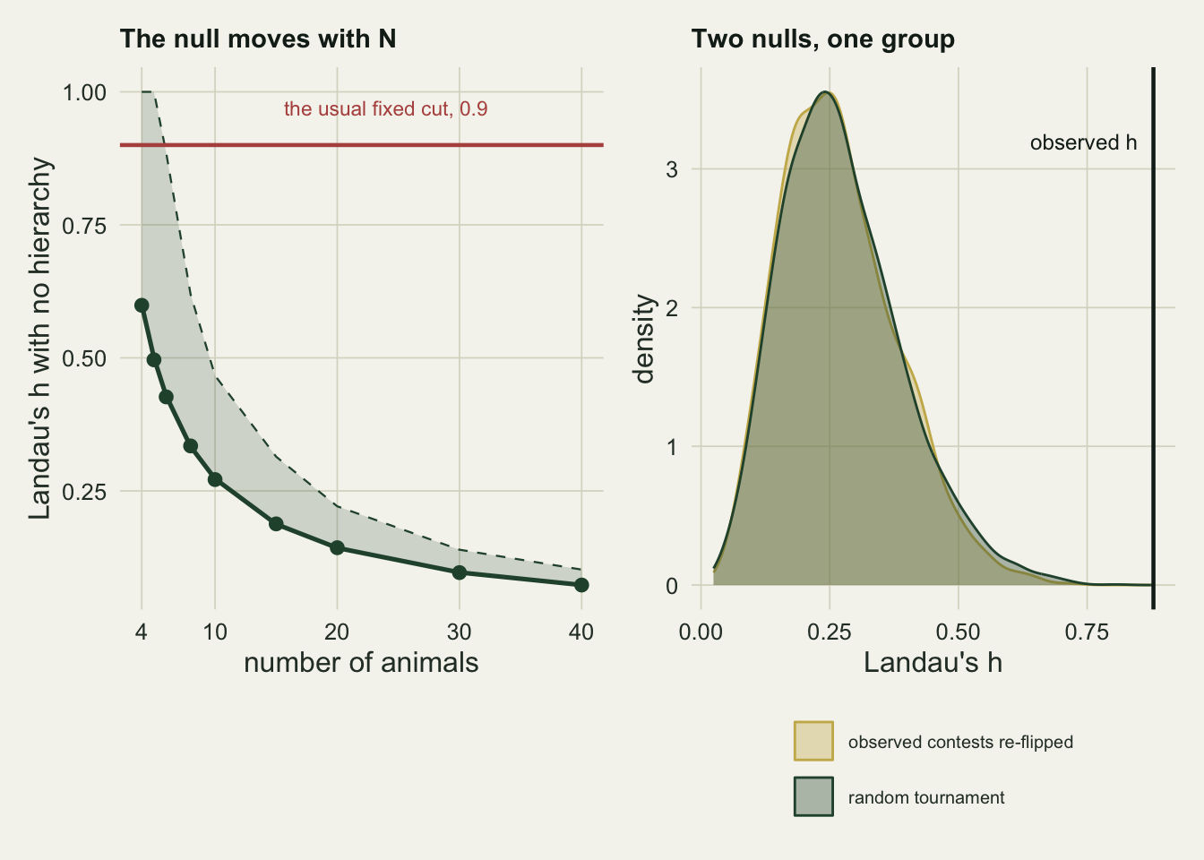
There is a second way to read h that makes the 3 / (N + 1) less mysterious. A triad is circular when A beats B, B beats C and C beats A. Writing d for the number of circular triads, h is exactly 1 - 24 d / (N^3 - N), so counting circular triads and computing h are one operation in two currencies; this group holds 5 circular triads out of 120, and putting that count through the identity returns 0.8788, matching the 0.8788 the win matrix gave to every digit printed. A triangle has three dyads and each can point two ways, which gives eight orientations, of which exactly two are circular. A quarter of all triads are circular under a fair coin, for every N and every group. Shizuka and McDonald’s triangle transitivity index is built on that quarter: it rescales the share of transitive triads so a random tournament sits at zero rather than at three quarters. Put the expected 30 circular triads through the identity and 3 / (N + 1) falls out.
Dyads nobody saw
Every pair in this group met at least once, which is a property of the simulation rather than of field data. In a real study many pairs are never seen interacting, and the linearity index still needs a number for those cells. The usual choice is the one that looks like no choice at all: leave the cell at zero, so neither animal beat the other.
That choice is not neutral, and the reason is arithmetic. When every pair is decided the V totals sum to N (N - 1) / 2 whoever won, and it is that fixed sum which holds h at or below 1. Code an unseen pair as a defeat for both animals and the sum falls, the mean V drops below the centre of the scale, and the squared deviations h adds up lose the bound that fixed sum gave them. The ceiling moves from 1 to 3 (N - 1) / (N + 1), which for a group this size is 2.4545, and it is reached when nothing was observed at all.
set.seed(3140)
n_rep_mis <- 400
frac_grid <- c(0, 0.1, 0.2, 0.3, 0.5, 0.7, 0.9)

n_unknown <- function(W) sum((W + t(W))[upper.tri(W)] == 0)
devries_h <- function(W) landau_h(W, unknown = 0.5) + 6 * n_unknown(W) / (n_ind^3 - n_ind)

thin_wins <- function(frac, flat) {
  ab <- if (flat) rep(0, n_ind) else ability
  u  <- round(frac * n_dyad)
  drop <- if (u > 0) sample(n_dyad, u) else integer(0)
  W <- matrix(0, n_ind, n_ind, dimnames = list(ids, ids))
  for (r in seq_len(n_dyad)) {
    if (r %in% drop) next
    i <- ij_all[r, 1]; j <- ij_all[r, 2]
    p <- 1 / (1 + exp(-(ab[i] - ab[j])))
    w <- rbinom(1, encounters[i, j], p)
    W[i, j] <- w; W[j, i] <- encounters[i, j] - w
  }
  W
}
miss_grid <- do.call(rbind, lapply(c(FALSE, TRUE), function(fl)
  do.call(rbind, lapply(frac_grid, function(f) {
    m <- t(vapply(seq_len(n_rep_mis), function(s) {
      W <- thin_wins(f, fl)
      c(landau_h(W, 0), landau_h(W, 0.5), devries_h(W))
    }, numeric(3)))
    data.frame(frac = f, flat = fl,
               coding = c("unseen coded 0/0", "unseen coded 0.5/0.5", "de Vries h'"),
               h = colMeans(m), se = apply(m, 2, sd) / sqrt(n_rep_mis))
  }))))
mis_se_max <- max(miss_grid$se)

pick_h <- function(fl, f, cd)
  miss_grid$h[miss_grid$flat == fl & miss_grid$frac == f & miss_grid$coding == cd]
frac_hi     <- 0.7
frac_top    <- 0.9
h0_hi_flat  <- pick_h(TRUE, frac_hi,  "unseen coded 0/0")
h0_top_flat <- pick_h(TRUE, frac_top, "unseen coded 0/0")
hp_top_flat <- pick_h(TRUE, frac_top, "de Vries h'")
lin_wins <- matrix(0, n_ind, n_ind, dimnames = list(ids, ids))
lin_wins[upper.tri(lin_wins)] <- 1
one_out <- vapply(seq_len(n_dyad), function(q) {
W <- lin_wins
W[ij_all[q, 1], ij_all[q, 2]] <- 0; W[ij_all[q, 2], ij_all[q, 1]] <- 0
landau_h(W)
}, numeric(1))
h_one_max <- max(one_out)
share_one_over <- mean(one_out > 1)It takes one unseen pair. Start from a perfectly linear group, delete a single one of its 45 dyads, and h reaches 1.0970; 22 per cent of the single deletions push it past 1. That check is exhaustive rather than sampled, since there are only 45 pairs to delete. An h above 1 is never a strong result. It says that something has been recorded as a defeat which was never a contest.
Sweeping the fraction of unseen dyads shows how far this runs, for the group in this post and for a group in which every animal is equally able.
miss_grid$panel  <- factor(ifelse(miss_grid$flat, "no hierarchy at all", "the group from this post"),
                           levels = c("the group from this post", "no hierarchy at all"))
miss_grid$coding <- factor(miss_grid$coding,
  levels = c("unseen coded 0/0", "unseen coded 0.5/0.5", "de Vries h'"))

ggplot(miss_grid, aes(100 * frac, h, colour = coding)) +
  geom_hline(yintercept = 1, colour = te_ink, linewidth = 0.6, linetype = "dashed") +
  geom_ribbon(aes(ymin = h - 2 * se, ymax = h + 2 * se, fill = coding), alpha = 0.25, colour = NA) +
  geom_line(linewidth = 0.9) +
  geom_point(size = 2) +
  annotate("text", x = 4, y = 1.08, label = "h = 1, the largest value a real order can give",
           hjust = 0, colour = te_ink, size = 3) +
  scale_colour_manual(values = c(te_rust, te_gold, te_forest), name = NULL) +
  scale_fill_manual(values = c(te_rust, te_gold, te_forest), name = NULL) +
  facet_wrap(~panel) +
  labs(x = "per cent of dyads never seen", y = "Landau's h",
       title = "Coding an unseen dyad as a double defeat manufactures linearity") +
  theme_datasheet() +
  theme(legend.position = "bottom",
        strip.text = element_text(colour = te_ink, face = "bold", size = 9))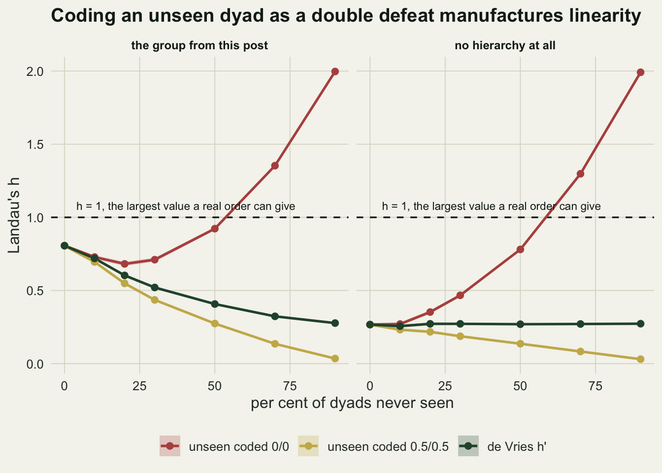
With 70 per cent of pairs never seen and no hierarchy at all, the zero coding reports 1.298, comfortably past a ceiling it should never reach, and at 90 per cent it reports 1.992. Nothing about the animals changed between those two numbers; only the share of cells that were filled in did.
de Vries’s repair is to impute an unseen pair as half a win each, which restores the fixed sum, and then to add back what the imputation removed: h’ is h computed that way plus 6 u / (N^3 - N) for u unknown pairs. The correction is chosen so the expected value under the coin flip null returns to 3 / (N + 1) however many pairs are missing, and it does. Across the same sweep with no hierarchy present h’ holds at 0.273 against the exact 0.2727, with a Monte Carlo standard error of at most 0.0070.
Missing dyads also decide which of the two nulls the randomisation test may use, and this is where the two stop agreeing.
set.seed(5527)
n_pick    <- 3000
frac_pick <- 0.5
drop_pick <- sample(n_dyad, round(frac_pick * n_dyad))
enc_pick  <- encounters
for (q in drop_pick) {
  enc_pick[ij_all[q, 1], ij_all[q, 2]] <- 0
  enc_pick[ij_all[q, 2], ij_all[q, 1]] <- 0
}
draw_flat <- function(E) {
  W <- matrix(0, n_ind, n_ind, dimnames = list(ids, ids))
  for (r in seq_len(n_dyad)) {
    i <- ij_all[r, 1]; j <- ij_all[r, 2]; k <- E[i, j]
    if (k == 0) next
    w <- rbinom(1, k, 0.5); W[i, j] <- w; W[j, i] <- k - w
  }
  W
}
h_pick_obs  <- landau_h(draw_flat(enc_pick))
h_pick_keep <- replicate(n_pick, landau_h(draw_flat(enc_pick)))
h_pick_full <- replicate(n_pick, landau_h(draw_flat(encounters)))
p_keep <- (sum(h_pick_keep >= h_pick_obs) + 1) / (n_pick + 1)
p_full <- (sum(h_pick_full >= h_pick_obs) + 1) / (n_pick + 1)
Take a group with no hierarchy at all, hide 50 per cent of its dyads, and code the gaps as zeros. Its h is 0.7273. The random tournament null, which quietly fills every pair back in, returns 0.0003. The null that keeps the observed design, leaving the unseen pairs unseen, returns 0.74 on the same number. The first would be written up as a strongly linear hierarchy in a group that has none, because it compares a statistic inflated by missingness against a null that has no missingness in it. Randomise the outcomes actually observed and leave the gaps where they are. The version that rebuilds a complete tournament is only safe when the tournament really was complete.
What to report
Give the encounter matrix, not only the ranking. The number of contests per dyad is what determines whether any of this is estimable, and it is one table.
Do not rank by proportion of wins. It is the only method here that gets the order wrong for a structural reason rather than a statistical one, and the structure is present in every observational dataset.
Fit Bradley-Terry with glm() and report the standard errors on the abilities. The design matrix takes a short loop over the observed pairs, the model is the same likelihood the specialist packages fit, and the errors tell you which adjacent ranks are not separated.
Run the strong connectivity test before trusting the fit. It costs one matrix power and it is the only reliable warning that the estimates are on their way to infinity.
If Elo is used, report the spread over random reorderings of the same contests, and the update constant. A single Elo ranking without both is one draw from a distribution the method does not show you.
Report a linearity index against its own null, never against a fixed cut. With no hierarchy at all the expected value of Landau’s h is 3 / (N + 1), so the same number is weak evidence in a small group and overwhelming in a large one. If any pair was never seen, report de Vries’s h’ and the count of unknown pairs beside it, because the uncorrected index climbs as the observation thins.
Honest limits
Everything here assumes a single fixed ability per animal for the whole observation period. Real hierarchies change: animals mature, alliances form, an alpha is deposed. Bradley-Terry and David’s score both average over that change and report something in the middle, while Elo tracks it, which is the one setting where Elo’s order dependence is a feature rather than a defect. Nothing in this post tests for a changing order, and the methods that do are a different exercise.
The simulation generates contests from exactly the Bradley-Terry model, so Bradley-Terry is being scored on its home ground. When real dominance is not transitive on a single latent scale, when A beats B, B beats C and C beats A reliably rather than by chance, no one-dimensional score describes it, and all four methods will return an order anyway. Counting circular triads is the check for that, and the linearity section above runs it in different units: 5 of this group’s 120 triads are circular.
The observed group has no unknown dyads: every pair meets at least once by construction, and the sweep above deletes pairs on purpose rather than meeting the gaps in the field. That is enough to show what the coding of an unseen pair does to the linearity index, and not enough to say what any of the four ranking scores would report on a genuinely sparse matrix. The chance corrected dyadic index handles rarely seen dyads but not unseen ones, and Bradley-Terry needs the digraph condition, which unseen dyads make much harder to satisfy.
The three hundred replicate summaries carry Monte Carlo error. The share of groups naming the wrong top animal has a standard error of at most 2.9 percentage points, so the wide gaps on that measure hold up, but the difference between the corrected David’s score and Bradley-Terry is not established by these runs.
The half win augmentation shown against separation is a demonstration, not a recommendation. It is a crude prior applied uniformly, it shrinks well estimated abilities as hard as unidentified ones, and the amount of shrinkage is a choice nobody has justified. Use it to see that the infinity is an artefact, then fit something with a stated prior.
References
David HA 1987 Biometrika 74(2):432-436 (10.1093/biomet/74.2.432)
Bradley RA, Terry ME 1952 Biometrika 39(3/4):324 (10.2307/2334029)
Sanchez-Tojar A, Schroeder J, Farine DR 2018 Journal of Animal Ecology 87(3):594-608 (10.1111/1365-2656.12776)
Landau HG 1951 Bulletin of Mathematical Biophysics 13(1):1-19 (10.1007/BF02478336)
de Vries H 1995 Animal Behaviour 50(5):1375-1389 (10.1016/0003-3472(95)80053-0)
Shizuka D, McDonald DB 2012 Animal Behaviour 83(4):925-934 (10.1016/j.anbehav.2012.01.011)