Permutation tests for social networks

Data-stream versus node permutation for animal social networks in R: the label shuffle inflates false positives to almost one, the pre-network null does not.

You have built a social network from group sightings. Now you want to test something: that individuals sort into preferred partners, or that bold animals sit at the centre, or that kin cluster together. Every one of those is a comparison against chance, and chance here means a null model: the networks that random association would produce. For animal social networks there are two popular nulls, they disagree, and picking the wrong one turns a sampling artefact into a publishable result.

Two shuffles

The node permutation shuffles the labels on the finished network. The edges stay exactly where they are; you just swap which individual sits at each node. It is quick, and it treats the network you measured as the ground truth.

The data-stream permutation goes back to the raw sightings. It swaps individuals between groups while keeping two things fixed: how many times each individual was seen, and how big each group was. Then it rebuilds the network from the shuffled sightings. Repeat that many times and you get the distribution of networks that random association would produce under your own sampling. It is slower, and it never trusts the observed network as more than one noisy draw.

Here is the machinery, all in base R. The network is a simple ratio index matrix; the metric we will test is degree, the number of distinct associates.

sri_from_gbi <- function(gbi) {
  co <- crossprod(gbi)
  n  <- diag(co)
  a  <- co / (outer(n, n, "+") - co)
  diag(a) <- 0
  a
}
node_degree <- function(a) rowSums(a > 0)

swap_data_stream <- function(gbi, n_swaps) {
  nr <- nrow(gbi); nc <- ncol(gbi); done <- 0L
  while (done < n_swaps) {
    batch <- (n_swaps - done) * 30L
    r1 <- sample.int(nr, batch, TRUE); r2 <- sample.int(nr, batch, TRUE)
    c1 <- sample.int(nc, batch, TRUE); c2 <- sample.int(nc, batch, TRUE)
    for (k in seq_len(batch)) {
      i1 <- r1[k]; i2 <- r2[k]; j1 <- c1[k]; j2 <- c2[k]
      if (i1 == i2 || j1 == j2) next
      if (gbi[i1,j1] && gbi[i2,j2] && !gbi[i1,j2] && !gbi[i2,j1]) {
        gbi[i1,j1] <- 0L; gbi[i2,j2] <- 0L; gbi[i1,j2] <- 1L; gbi[i2,j1] <- 1L
        done <- done + 1L
      } else if (gbi[i1,j2] && gbi[i2,j1] && !gbi[i1,j1] && !gbi[i2,j2]) {
        gbi[i1,j2] <- 0L; gbi[i2,j1] <- 0L; gbi[i1,j1] <- 1L; gbi[i2,j2] <- 1L
        done <- done + 1L
      }
      if (done == n_swaps) break
    }
  }
  gbi
}

The swap flips a two by two block of the group-by-individual matrix: individual A leaves one group and joins another while individual B does the reverse. That move keeps every row sum and every column sum intact, which is what “keep the sampling fixed” means in practice.

The degenerate case: testing for preferred associations

The classic question is whether a society has preferred and avoided companions at all. The standard statistic is the coefficient of variation of the association indices: a well-mixed society gives similar weights everywhere (low CV), a differentiated one gives a mix of strong and weak bonds (high CV). You compare the observed CV to a null.

Try to build that null by relabelling nodes and watch it collapse.

set.seed(1)
m <- matrix(runif(15 * 15), 15, 15); m <- (m + t(m)) / 2; diag(m) <- 0
cv <- function(a) { v <- a[upper.tri(a)]; sd(v) / mean(v) }
obs_cv <- cv(m)
relabel_cv <- replicate(2000, { p <- sample(15); cv(m[p, p]) })
c(observed = round(obs_cv, 4),
  null_min = round(min(relabel_cv), 4),
  null_max = round(max(relabel_cv), 4),
  null_sd  = signif(sd(relabel_cv), 3))

 observed  null_min  null_max   null_sd 
3.869e-01 3.869e-01 3.869e-01 6.290e-17 

The null minimum, maximum and observed value are the same number, and the null standard deviation is zero. This is not bad luck; it is arithmetic. Relabelling the nodes shuffles the rows and columns of the matrix together, so the set of edge weights never changes, so its coefficient of variation never changes. A node permutation cannot test the CV, because the CV is blind to who sits where. For this question you have no choice: the null has to come from the data stream, which reshuffles the sightings and can produce genuinely different sets of weights.

The inflated case: does a trait predict position?

The subtler failure is the one that looks like it works. Suppose you test whether a trait predicts a node metric, and the trait happens to correlate with how often the individual was seen. That is common: bolder animals, or those carrying a working tag, or those living near the road, are simply observed more.

Build one such dataset. Association is entirely random here (no preferences), individuals differ only in sighting frequency, and the “trait” is nothing but a noisy copy of the sighting count. To make the observed network a clean draw from random association, generate it by starting from independent sightings and mixing with a long run of swaps.

set.seed(27)
n_ind <- 20; n_grp <- 24
detect <- runif(n_ind, 0.10, 0.35)
raw <- matrix(rbinom(n_grp * n_ind, 1, rep(detect, each = n_grp)), n_grp, n_ind)
raw <- raw[rowSums(raw) > 0, ]
raw <- raw[, colSums(raw) > 0]
gbi <- swap_data_stream(raw, 1500)               # a random-association network
trait <- colSums(gbi) + rnorm(ncol(gbi), 0, 1.2) # trait tracks sighting count only
net  <- sri_from_gbi(gbi)
deg  <- node_degree(net)
obs_r <- cor(trait, deg)

n_perm <- 1000
node_null <- replicate(n_perm, cor(sample(trait), deg))
p_node <- mean(abs(node_null) >= abs(obs_r))

ds_null <- numeric(n_perm); g <- gbi
for (b in seq_len(n_perm)) {
  g <- swap_data_stream(g, 50)
  ds_null[b] <- cor(trait, node_degree(sri_from_gbi(g)))
}
p_ds <- mean(abs(ds_null) >= abs(obs_r))

c(observed_cor = round(obs_r, 3),
  p_node = round(p_node, 3),
  p_data_stream = round(p_ds, 3),
  cor_trait_count  = round(cor(trait, colSums(gbi)), 3),
  cor_degree_count = round(cor(deg, colSums(gbi)), 3))

    observed_cor           p_node    p_data_stream  cor_trait_count 
           0.808            0.000            0.632            0.930 
cor_degree_count 
           0.852 

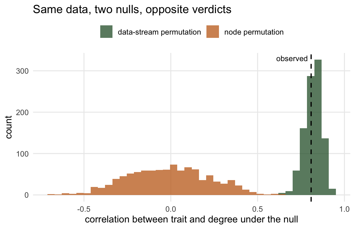
Read the output straight down: the observed correlation between trait and degree is strong, the node permutation returns a p-value of essentially zero, and the data-stream permutation returns a large one. Both nulls saw the same data. One screams significance, the other shrugs. The two extra numbers explain why: the trait tracks sighting count almost perfectly, and degree tracks sighting count almost as tightly. There is no social story here, only a sampling one.

The picture shows what each null is comparing against.

nulls <- rbind(
  data.frame(r = node_null, null = "node permutation"),
  data.frame(r = ds_null,   null = "data-stream permutation"))
ggplot(nulls, aes(r, fill = null)) +
  geom_histogram(bins = 40, alpha = 0.75, position = "identity") +
  geom_vline(xintercept = obs_r, linetype = "dashed", linewidth = 0.7) +
  annotate("text", x = obs_r, y = Inf, label = "observed", vjust = 1.5, hjust = 1.1, size = 3.4) +
  scale_fill_manual(values = c("node permutation" = "#c46a1b",
                               "data-stream permutation" = "#2b5d34"), name = NULL) +
  labs(title = "Same data, two nulls, opposite verdicts",
       x = "correlation between trait and degree under the null", y = "count") +
  theme(legend.position = "top")

Figure 1: The observed correlation against two null distributions. The node permutation sits at zero, so the observed value looks extreme. The data-stream null sits where sampling puts it, and the observed value is an ordinary member of it.

How often does each null cry wolf?

One dataset is an anecdote. The honest measure is the false-positive rate: run many datasets where association is random, and count how often each test rejects at the five percent level. A calibrated test should reject about five percent of the time. Anything much higher is manufacturing significance.

one_study <- function(n_ind = 20, n_grp = 24, n_perm = 120, n_sw = 50, burn = 1500) {
  d <- runif(n_ind, 0.10, 0.35)
  g0 <- matrix(rbinom(n_grp * n_ind, 1, rep(d, each = n_grp)), n_grp, n_ind)
  g0 <- g0[rowSums(g0) > 0, ]; g0 <- g0[, colSums(g0) > 0]
  gbi <- swap_data_stream(g0, burn)
  trait <- colSums(gbi) + rnorm(ncol(gbi), 0, 1.2)
  deg <- node_degree(sri_from_gbi(gbi))
  if (sd(deg) == 0) return(c(NA, NA))
  obs <- cor(trait, deg)
  nn <- replicate(n_perm, cor(sample(trait), deg))
  p_node <- mean(abs(nn) >= abs(obs))
  dd <- numeric(n_perm); g <- gbi
  for (b in seq_len(n_perm)) {
    g <- swap_data_stream(g, n_sw); dg <- node_degree(sri_from_gbi(g))
    dd[b] <- if (sd(dg) == 0) NA else cor(trait, dg)
  }
  c(p_node = p_node, p_ds = mean(abs(dd) >= abs(obs), na.rm = TRUE))
}

set.seed(2024)
res <- t(replicate(120, one_study()))
res <- res[!is.na(res[, 1]), ]
se <- function(p, n) sqrt(p * (1 - p) / n)
rate_node <- mean(res[, "p_node"] < 0.05)
rate_ds   <- mean(res[, "p_ds"]   < 0.05)
c(studies = nrow(res),
  node_type_I_pct = round(100 * rate_node, 1),
  node_SE = round(100 * se(rate_node, nrow(res)), 1),
  data_stream_type_I_pct = round(100 * rate_ds, 1),
  data_stream_SE = round(100 * se(rate_ds, nrow(res)), 1))

               studies        node_type_I_pct                node_SE 
                 120.0                   99.2                    0.8 
data_stream_type_I_pct         data_stream_SE 
                   1.7                    1.2 

The node permutation rejects almost every time: a false-positive rate near one hundred percent when it should be five. The data-stream permutation lands close to the nominal five percent (a little under, which is the safe direction). Over these Monte Carlo runs the standard errors are a percentage point or two, so the gap is not noise. If you had used the node permutation on random data, you would have “discovered” that your trait drives social position in almost every study you ran.

Why the label shuffle fails

The node permutation is not wrong in general. It is the right null when the network is measured without error, so that the only randomness left is the assignment of traits to fixed nodes. Genetic relatedness on a known pedigree, or an experimentally imposed treatment, fit that description.

An observation-derived social network does not. It is a noisy, sampling-shaped object: watch an individual more and it accumulates more edges, higher degree, more chances to look central, whatever its true sociality. The node permutation freezes that artefact into the null and then measures your trait against it, so any trait that also tracks sampling sails through. The data-stream permutation rebuilds the network from scratch under random association, carrying the same sighting counts and group sizes, so the artefact appears in the null too and stops counting as signal.

The honest limit

The data-stream null is only as good as the constraints it preserves. Keeping sighting counts and group sizes fixed handles the frequency artefact shown here, but real sampling has more structure: sightings clumped in time, uneven coverage across sites, demographic turnover. If those matter for your question and your permutation ignores them, the data-stream null can be miscalibrated in its own way; you may need to restrict swaps within days, sites, or periods. The method is not a black box that launders any dataset. It is a way of encoding what you believe random association would look like given how you actually watched, and that belief is yours to state and defend.

With a null you can trust, the next post turns the network into per-individual scores and shows that the same sampling artefact haunts them too.

Where to go next

The centrality post computes degree, strength and eigenvector centrality and asks what each one means once you know that sighting effort inflates all of them. The checking post makes the false-positive risk, the power to detect real structure, and the group-definition assumption into a short diagnostic routine. If you built the network by a different route, the association-index post covers where the edge weights came from.

Related tutorials

• Association indices for social networks
• Network centrality and sampling effort
• Checking a social network analysis
• Null models for interaction networks

References

Bejder L, Fletcher D, Brager S 1998 Animal Behaviour 56(3):719-725 (10.1006/anbe.1998.0802)

Whitehead H 1999 Animal Behaviour 57:F26-F29 (10.1006/anbe.1999.1099)

Farine DR 2017 Methods in Ecology and Evolution 8(10):1309-1320 (10.1111/2041-210X.12772)

Farine DR, Whitehead H 2015 Journal of Animal Ecology 84(5):1144-1163 (10.1111/1365-2656.12418)