Interaction rewiring and its sampling floor

Two samples of one pollination web differ, and Poisot’s partition calls that rewiring. The sampling floor in closed form, and a permutation test on bouts.

A meadow has been watched for two summers. Each year a team walked the same transects, recorded every insect seen touching the anthers or stigma of a flower, and ended with a plant by pollinator matrix of a few thousand records. The two matrices are not the same. Some bees were seen in one year only, and among the species seen in both years many links appear once and not the other time. The analysis that has become routine for this comparison is the partition of Poisot and colleagues (2012): total interaction dissimilarity between the two webs, beta_WN, is split into a part due to species turnover and a part, beta_OS, computed on the species present in both webs and read as rewiring, the same species interacting with different partners. CaraDonna and colleagues (2017) built networks from weekly censuses and found that week to week turnover was dominated by rewiring.

The partition has two known problems, and this post demonstrates both rather than discovering either. Frund (2021) showed that the commonly used form, where beta_OS gets its own denominator and species turnover is whatever is left over, overstates the rewiring share, and he recommended a partition in which both components share the denominator of beta_WN. And the matrices are samples. Frund, McCann and Williams (2016) showed how far network indices move with sampling effort on a single web; two samples of one unchanging web also differ, and every link seen in only one of them counts towards beta_OS.

The single-web version of the sampling problem is already on this site. Checking a network analysis samples one known web at rising effort and watches connectance, H2’ and nestedness drift, and its last section separates forbidden links from missed ones. Null models for interaction networks shuffles one matrix to ask what a metric would be by chance. Neither compares two webs. The comparison is the subject here, and the lesson it ends on is the one permutation tests for social networks teaches for association data: the result depends on choosing the unit that is exchangeable under the null, and for pollination records that unit is the foraging visit, not the record.

The post does four things. It writes the expected rewiring component of two samples of one web in closed form and checks it against simulation. It shows that pure species loss leaves that floor almost where it was, so the share called rewiring is set by effort, under both partitions. It builds a permutation test that asks whether beta_OS exceeds what two samples of one web give. Then it breaks that test with records that arrive in foraging bouts, repairs it by permuting bouts, and shows that this repair breaks again when bout length differs between years, unless bouts are shuffled only among bouts of the same length.

library(ggplot2)
library(patchwork)

te_paper  <- "#f5f4ee"
te_ink    <- "#16241d"
te_body   <- "#2c3a31"
te_forest <- "#275139"
te_rust   <- "#b5534e"
te_gold   <- "#c9b458"
te_line   <- "#dad9ca"

theme_datasheet <- function() {
  theme_minimal(base_size = 12) +
    theme(plot.background  = element_rect(fill = te_paper, colour = NA),
          panel.background = element_rect(fill = te_paper, colour = NA),
          panel.grid.major = element_line(colour = te_line, linewidth = 0.3),
          panel.grid.minor = element_blank(),
          text             = element_text(colour = te_body),
          plot.title       = element_text(colour = te_ink, face = "bold"),
          plot.subtitle    = element_text(colour = te_body),
          axis.text        = element_text(colour = te_body))
}

Two samples of one web

The simulated web has 25 plant species and 40 pollinator species. Each species has a trait on the unit interval and an activity drawn from a lognormal distribution, and the probability that a record falls in a cell is the product of the two activities times a Gaussian trait matching term of width 0.15. A sample of m records is a multinomial draw from those cell probabilities. That gives a web with a few very common links, a long tail of rare ones, and a set of trait combinations that almost never meet.

Two changes can be imposed on the second year. Species loss removes a fixed fraction of pollinator columns and renormalises. Rewiring gives a fixed fraction of pollinator species a new trait value, so they keep their activity and move to other plants. Both are design constants fixed before any of the runs below.

The partition follows the two published forms. In Poisot’s form beta_WN is the Sorensen dissimilarity of the two binary link sets, beta_OS is the same index computed on the sub-web of plants and pollinators detected in both years, and species turnover is the difference. In the common denominator form that Frund recommends, the links that differ between years are split into those among shared species and the rest, and both counts are divided by the denominator of beta_WN, so the two parts add up by construction.

n_plant <- 25
n_poll  <- 40
match_w <- 0.15
n_cell  <- n_plant * n_poll
row_id  <- rep(seq_len(n_plant), times = n_poll)
col_id  <- rep(seq_len(n_poll), each = n_plant)

make_web <- function() {
  list(trait_p = runif(n_plant), trait_a = runif(n_poll),
       act_p = rlnorm(n_plant), act_a = rlnorm(n_poll))
}
web_prob <- function(w) {
  cell <- outer(w$act_p, w$act_a) *
    exp(-outer(w$trait_p, w$trait_a, "-")^2 / (2 * match_w^2))
  as.vector(cell / sum(cell))
}
make_pair <- function(loss, rewire) {
  w1 <- make_web()
  w2 <- w1
  if (rewire > 0) {
    moved <- sample(n_poll, round(rewire * n_poll))
    w2$trait_a[moved] <- runif(length(moved))
  }
  p1 <- web_prob(w1)
  p2 <- web_prob(w2)
  if (loss > 0) {
    lost <- sample(n_poll, round(loss * n_poll))
    p2[col_id %in% lost] <- 0
    p2 <- p2 / sum(p2)
  }
  list(p1 = p1, p2 = p2)
}
draw_counts <- function(p, m) as.vector(rmultinom(1, m, p))

partition <- function(x1, x2) {
  seen1 <- x1 > 0
  seen2 <- x2 > 0
  n_both <- sum(seen1 & seen2)
  n_diff <- sum(seen1 != seen2)
  denom  <- 2 * n_both + n_diff
  row_sh <- tabulate(row_id[seen1], n_plant) > 0 & tabulate(row_id[seen2], n_plant) > 0
  col_sh <- tabulate(col_id[seen1], n_poll) > 0 & tabulate(col_id[seen2], n_poll) > 0
  shared <- row_sh[row_id] & col_sh[col_id]
  both_sh <- sum(seen1 & seen2 & shared)
  diff_sh <- sum((seen1 != seen2) & shared)
  sp_same <- all((tabulate(row_id[seen1], n_plant) > 0) == (tabulate(row_id[seen2], n_plant) > 0)) &&
    all((tabulate(col_id[seen1], n_poll) > 0) == (tabulate(col_id[seen2], n_poll) > 0))
  c(wn = n_diff / denom,
    os_poisot = diff_sh / (2 * both_sh + diff_sh),
    os_common = diff_sh / denom,
    same_species = sp_same)
}

For an unchanging web the expected dissimilarity can be written down before anything is simulated. A cell with probability q is detected in a sample of m records with probability p = 1 - (1 - q)^m, independently in the two samples. It is seen in both with probability p squared and in exactly one with probability 2p(1 - p). Putting the expected counts into the Sorensen form gives the floor sum p(1 - p) / sum p, a ratio of expectations that should sit close to the mean ratio once the web has more than a handful of detectable links. When both samples detect the same species, beta_OS and beta_WN are the same number, so the same floor is the expected rewiring component. None of this needs a named source; it is detection arithmetic, and the point of computing it is that the simulated floor below should not be read as a surprise.

efforts  <- c(200, 500, 1000, 3000, 10000)
n_pair   <- 200
loss_use <- 0.3

floor_cf <- function(p, m) {
  detect <- 1 - (1 - p)^m
  sum(detect * (1 - detect)) / sum(detect)
}

set.seed(20917)
grid_list <- list()
for (m_eff in efforts) {
  for (loss in c(0, loss_use)) {
    out <- replicate(n_pair, {
      pr <- make_pair(loss, 0)
      c(partition(draw_counts(pr$p1, m_eff), draw_counts(pr$p2, m_eff)),
        closed = floor_cf(pr$p1, m_eff))
    })
    grid_list[[length(grid_list) + 1]] <- data.frame(
      effort = m_eff, loss = loss,
      wn = mean(out["wn", ]), os_poisot = mean(out["os_poisot", ]),
      os_common = mean(out["os_common", ]),
      os_se = sd(out["os_poisot", ]) / sqrt(n_pair),
      same_species = mean(out["same_species", ]),
      closed = mean(out["closed", ]))
  }
}
floor_tab <- do.call(rbind, grid_list)
floor_tab$share_poisot <- floor_tab$os_poisot / floor_tab$wn
floor_tab$share_common <- floor_tab$os_common / floor_tab$wn

pick <- function(col, m_eff, loss) floor_tab[[col]][floor_tab$effort == m_eff & floor_tab$loss == loss]
cf_diff <- floor_tab$closed - floor_tab$os_poisot
cf_gap_hi <- max(abs(cf_diff)[floor_tab$loss == 0 & floor_tab$effort >= 1000])
cf_gap_500 <- cf_diff[floor_tab$loss == 0 & floor_tab$effort == 500]
cf_gap_200 <- cf_diff[floor_tab$loss == 0 & floor_tab$effort == 200]
round(floor_tab[, c("effort", "loss", "wn", "os_poisot", "closed", "share_poisot", "share_common")], 3)

   effort loss    wn os_poisot closed share_poisot share_common
1     200  0.0 0.532     0.498  0.535        0.937        0.875
2     200  0.3 0.598     0.489  0.536        0.818        0.643
3     500  0.0 0.399     0.389  0.401        0.975        0.959
4     500  0.3 0.485     0.376  0.398        0.774        0.636
5    1000  0.0 0.309     0.306  0.307        0.990        0.985
6    1000  0.3 0.411     0.291  0.308        0.708        0.587
7    3000  0.0 0.191     0.191  0.191        0.998        0.998
8    3000  0.3 0.318     0.180  0.191        0.566        0.470
9   10000  0.0 0.109     0.109  0.109        1.000        1.000
10  10000  0.3 0.259     0.107  0.112        0.412        0.341

On the unchanging web, beta_OS averages 0.498 at 200 records per year, 0.389 at 500, 0.191 at 3000 and 0.109 at 10000. The closed form, computed on the same simulated webs, gives 0.535, 0.401, 0.191 and 0.109. From 1000 records upward the two differ by at most 0.002, against a Monte Carlo standard error of the simulated mean of at most 0.004. At 500 records the closed form is 0.012 above the simulation and at 200 records 0.037 above it, because beta_OS is computed only on species detected in both samples, and at low effort many rare species are not, so their unmatched links drop out of the sub-web.

The same fact makes the rewiring share of an unchanging web uninformative. The share beta_OS / beta_WN is 0.975 at 500 records and 0.998 at 3000, but at 3000 records the two samples detect exactly the same species in 0.89 of pairs, and in those pairs the share is one by definition. Nothing about rewiring is learned from it. What the unchanging web does give is the size of the floor: at 3000 records per year, which is a substantial field season, about a fifth of the links among shared species differ between two samples of the same web.

floor_long <- rbind(
  data.frame(effort = floor_tab$effort[floor_tab$loss == 0],
             value = floor_tab$os_poisot[floor_tab$loss == 0],
             series = "beta_OS, unchanging web"),
  data.frame(effort = floor_tab$effort[floor_tab$loss == loss_use],
             value = floor_tab$os_poisot[floor_tab$loss == loss_use],
             series = "beta_OS, 30 per cent of pollinators lost"),
  data.frame(effort = floor_tab$effort[floor_tab$loss == loss_use],
             value = floor_tab$wn[floor_tab$loss == loss_use],
             series = "beta_WN, 30 per cent of pollinators lost"))
cf_line <- data.frame(effort = floor_tab$effort[floor_tab$loss == 0],
                      value = floor_tab$closed[floor_tab$loss == 0])

ggplot(floor_long, aes(effort, value)) +
  geom_line(data = cf_line, colour = te_ink, linetype = "dashed", linewidth = 0.7) +
  geom_line(aes(colour = series), linewidth = 0.9) +
  geom_point(aes(colour = series), size = 2.4) +
  scale_colour_manual(values = c(te_forest, te_gold, te_rust), name = NULL) +
  scale_x_log10(breaks = efforts) +
  scale_y_continuous(limits = c(0, NA)) +
  guides(colour = guide_legend(ncol = 1)) +
  labs(x = "records per year (log scale)", y = "dissimilarity",
       title = "A floor that only effort lowers",
       subtitle = "dashed: closed form sum p(1 - p) / sum p for the unchanging web") +
  theme_datasheet() +
  theme(legend.position = "bottom")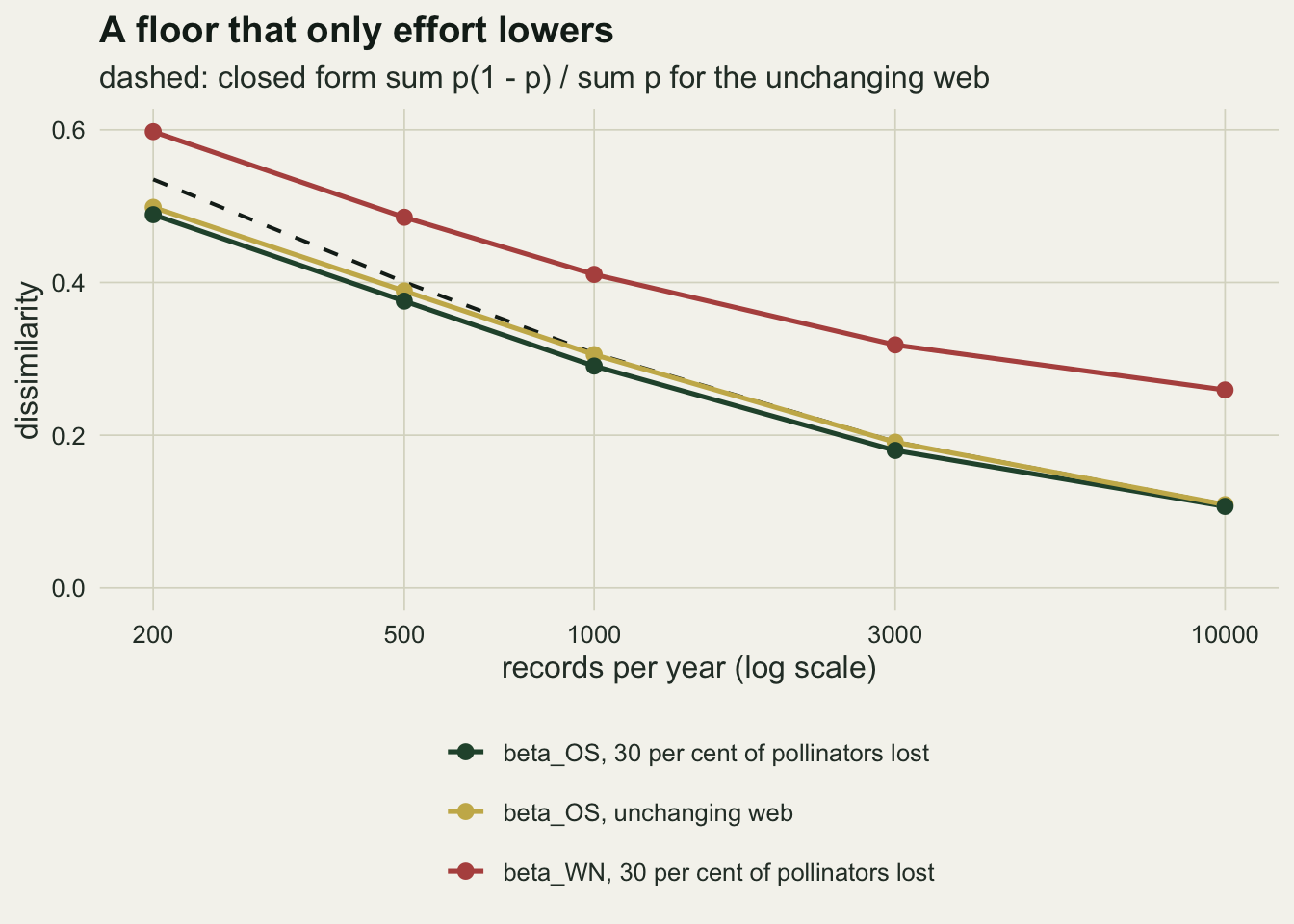

Figure 1: The rewiring component of two samples of one unchanging web, simulated and in closed form, and the same component when 30 per cent of the pollinator species are lost.

Species loss moves the total, not the floor

Now let the second year lose 30 per cent of its pollinator species, and nothing else. There is no rewiring in this scenario: every surviving species keeps exactly the partners it had. With complete sampling the rewiring component would be zero and all of the dissimilarity would be species turnover.

With 500 records per year, beta_WN rises from 0.399 to 0.485, while beta_OS is 0.376 against 0.389 on the unchanging web. At 10000 records the pair is 0.107 against 0.109. The species that remain are sampled at the same depth as before, so their sub-web carries the same floor, a little lower because the surviving species receive the records that the lost ones no longer take. The share called rewiring is then the floor divided by the total, and it falls only because the total stays up while the floor comes down with effort: 0.77 at 500 records, 0.57 at 3000 and 0.41 at 10000, in a scenario whose true share is zero.

Frund’s common denominator form changes the share but not the pattern. Its rewiring share under pure species loss is 0.64 at 500 records, 0.47 at 3000 and 0.34 at 10000. It is lower than Poisot’s share at every effort, which is the direction Frund reported, and at every effort it is still far above zero. The lower share does not make the common denominator form free of the problem. The choice of denominator and the sampling floor are separate issues: the denominator scales the floor, and only effort removes it.

set.seed(41)
rare_out <- replicate(n_pair, {
  pr <- make_pair(0, 0)
  x_small <- draw_counts(pr$p1, 500)
  x_large <- draw_counts(pr$p2, 1500)
  keep <- sample(rep.int(seq_len(n_cell), x_large), 500)
  x_rare <- tabulate(keep, n_cell)
  c(unequal = partition(x_small, x_large)[["os_poisot"]],
    rarefied = partition(x_small, x_rare)[["os_poisot"]])
})
rare_mean <- rowMeans(rare_out)

A common reflex when the two years differ in effort is to rarefy the larger web to the smaller total before comparing. On the unchanging web with 500 records in one year and 1500 in the other, beta_OS averages 0.370; after rarefying the larger year to 500 records it averages 0.388, which is the equal effort floor at 500 records from the grid above, 0.389. Rarefying moved beta_OS up, not down, and the equality has to hold, because subsampling a multinomial sample without replacement gives another multinomial sample of the smaller size. Rarefying makes the two years comparable with each other; it returns the comparison to the floor of the smaller year and does not take it below.

share_df <- rbind(
  data.frame(effort = floor_tab$effort[floor_tab$loss == loss_use],
             share = floor_tab$share_poisot[floor_tab$loss == loss_use],
             form = "Poisot: beta_OS on its own denominator"),
  data.frame(effort = floor_tab$effort[floor_tab$loss == loss_use],
             share = floor_tab$share_common[floor_tab$loss == loss_use],
             form = "Common denominator (Frund 2021)"))

ggplot(share_df, aes(effort, share, colour = form)) +
  geom_hline(yintercept = 0, colour = te_ink, linewidth = 0.6) +
  geom_line(linewidth = 0.9) +
  geom_point(size = 2.4) +
  scale_colour_manual(values = c(te_forest, te_rust), name = NULL) +
  scale_x_log10(breaks = efforts) +
  scale_y_continuous(limits = c(0, 1)) +
  guides(colour = guide_legend(ncol = 1)) +
  labs(x = "records per year (log scale)", y = "share of beta_WN called rewiring",
       title = "Pure species loss, read as rewiring",
       subtitle = "the true share in this scenario is zero (solid line)") +
  theme_datasheet() +
  theme(legend.position = "bottom")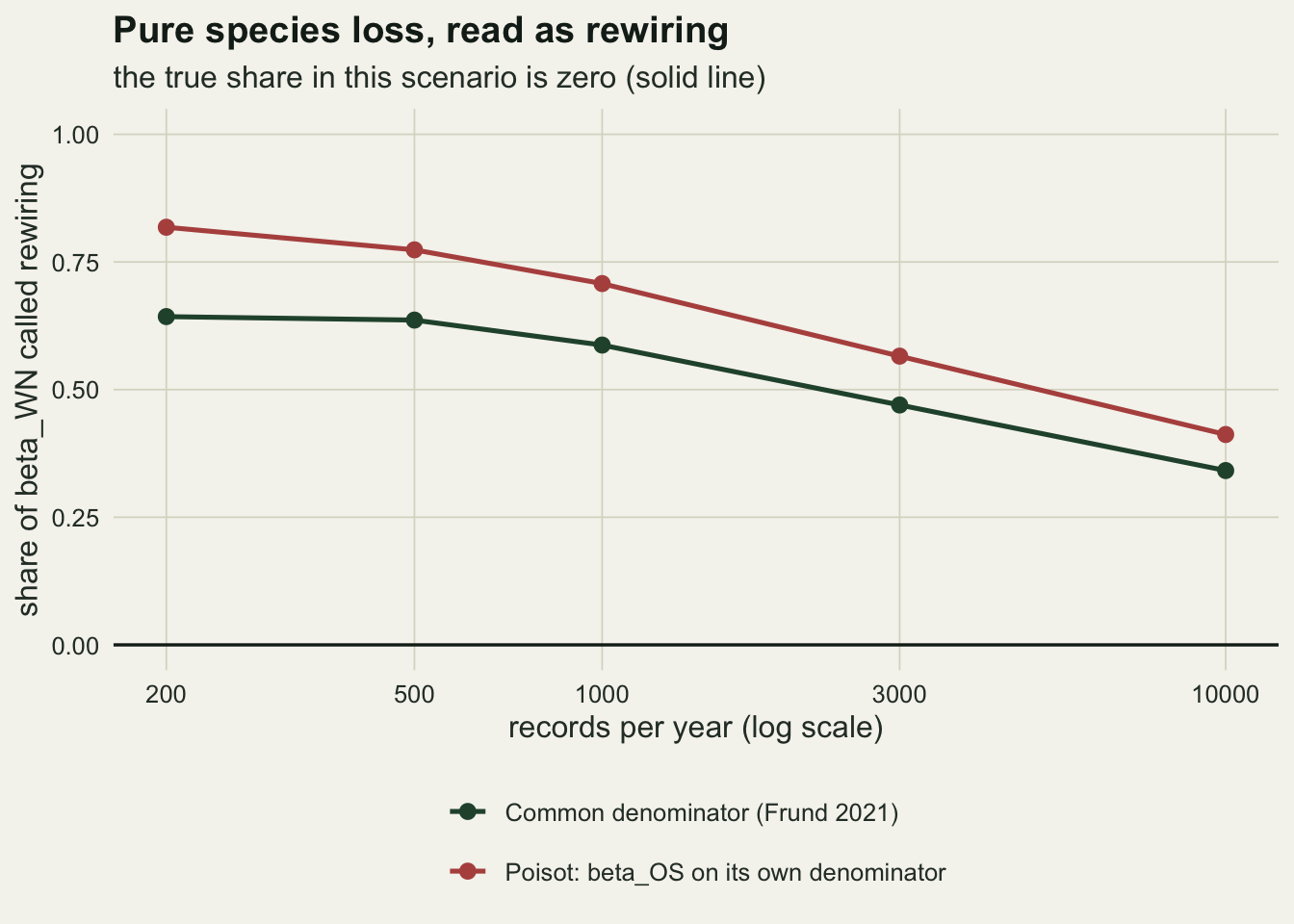

Figure 2: Share of dissimilarity called rewiring when 30 per cent of the pollinator species are lost and nobody rewires, under Poisot’s partition and the common denominator partition.

A permutation of records asks the right question

The partition cannot say whether beta_OS is larger than sampling alone would make it. A permutation can. If both years are samples of one web, then the pooled records could have fallen in either year, and shuffling them between years while keeping each year’s total gives the distribution of beta_OS under that null, at the observed effort and on the observed mix of common and rare links. The test is one sided: rewiring shows up as more dissimilarity among shared species than the shuffled pairs produce. Nothing about the null needs the true web, and the floor is built into it automatically.

The replication for all tests was fixed before running at 200 pairs of webs per cell and 99 permutations per pair, so a rejection rate near the nominal five per cent has a Monte Carlo standard error of 0.015, and no rate has one above 0.035.

n_test <- 200
n_perm <- 99
mc_se_05 <- sqrt(0.05 * 0.95 / n_test)

os_cells <- function(cells1, cells2) {
  seen1 <- tabulate(cells1, n_cell) > 0
  seen2 <- tabulate(cells2, n_cell) > 0
  row_sh <- tabulate(row_id[seen1], n_plant) > 0 & tabulate(row_id[seen2], n_plant) > 0
  col_sh <- tabulate(col_id[seen1], n_poll) > 0 & tabulate(col_id[seen2], n_poll) > 0
  shared <- row_sh[row_id] & col_sh[col_id]
  diff_sh <- sum((seen1 != seen2) & shared)
  both_sh <- sum(seen1 & seen2 & shared)
  if (diff_sh + both_sh == 0) return(0)
  diff_sh / (2 * both_sh + diff_sh)
}
perm_records <- function(cells1, cells2, nperm = n_perm) {
  obs  <- os_cells(cells1, cells2)
  pool <- c(cells1, cells2)
  n1   <- length(cells1)
  null_os <- vapply(seq_len(nperm), function(i) {
    shuffled <- sample(pool)
    os_cells(shuffled[seq_len(n1)], shuffled[-seq_len(n1)])
  }, numeric(1))
  (1 + sum(null_os >= obs)) / (nperm + 1)
}
draw_cells <- function(p, m) sample.int(n_cell, m, replace = TRUE, prob = p)

scen_tab <- data.frame(scenario = c("unchanging", "species loss only",
                                    "rewiring 15 per cent", "rewiring 30 per cent"),
                       loss = c(0, loss_use, 0, 0), rewire = c(0, 0, 0.15, 0.3))
set.seed(3203)
rec_list <- list()
for (m_eff in c(500, 3000)) {
  for (k in seq_len(nrow(scen_tab))) {
    p_val <- replicate(n_test, {
      pr <- make_pair(scen_tab$loss[k], scen_tab$rewire[k])
      perm_records(draw_cells(pr$p1, m_eff), draw_cells(pr$p2, m_eff))
    })
    rec_list[[length(rec_list) + 1]] <- data.frame(
      effort = m_eff, scenario = scen_tab$scenario[k], reject = mean(p_val <= 0.05))
  }
}
rec_tab <- do.call(rbind, rec_list)
rpick <- function(m_eff, scen) rec_tab$reject[rec_tab$effort == m_eff & rec_tab$scenario == scen]
rec_tab

  effort             scenario reject
1    500           unchanging  0.045
2    500    species loss only  0.045
3    500 rewiring 15 per cent  0.520
4    500 rewiring 30 per cent  0.865
5   3000           unchanging  0.040
6   3000    species loss only  0.055
7   3000 rewiring 15 per cent  0.930
8   3000 rewiring 30 per cent  1.000

With independent records the test holds its level. On unchanging webs it rejects in 0.045 of pairs at 500 records per year and 0.040 at 3000. Under species loss with no rewiring it rejects in 0.045 and 0.055; beta_OS is computed on shared species, and the loss of species does not raise it above the floor, as the grid showed. When 30 per cent of pollinator species move to new partners, the rejection rate is 0.865 at 500 records and 1.000 at 3000; for 15 per cent it is 0.520 and 0.930.

The test does not say how much of the turnover is rewiring. It says whether the rewiring component is more than two samples of one web would show, which is the question a two year comparison has to answer first.

Records that arrive in bouts

The permutation above treats every record as an independent draw from the web. Field records are not collected that way. A bumblebee that lands in a patch of knapweed works several flower heads before it leaves, and a transect protocol that logs each flower visit writes that one foraging decision into the matrix several times. The records within a bout share a pollinator, and often a plant.

The bout generator below draws a pollinator for each bout in proportion to its activity, then visits a fixed number of flowers. The first plant is drawn from that pollinator’s row of partner probabilities; each later flower is the same plant as the previous one with a constancy probability, and otherwise a fresh draw. Two years with 200 bouts of 6 flower visits each give 1200 records per year, and the main arm uses full constancy, one plant per bout, which is the extreme case. A constancy of one half is run as well.

The bout permutation keeps the bout intact. It shuffles whole bouts between years, keeping the number of bouts in each year, and rebuilds both webs from the shuffled bouts. Under the null that both years are samples of one web, bouts are exchangeable between years in the way records are not.

bout_len  <- 6
n_bout    <- 200

draw_bouts <- function(p, nb, lens, constancy) {
  cell_mat <- matrix(p, n_plant, n_poll)
  col_mass <- colSums(cell_mat)
  poll <- sample.int(n_poll, nb, replace = TRUE, prob = col_mass)
  cum_plant <- apply(sweep(cell_mat, 2, col_mass, "/"), 2, cumsum)
  pick_plant <- function(pl) {
    u <- runif(length(pl))
    pmin(1 + rowSums(u > t(cum_plant[, pl, drop = FALSE])), n_plant)
  }
  kmax <- max(lens)
  plants <- matrix(0L, nb, kmax)
  plants[, 1] <- pick_plant(poll)
  if (kmax > 1) {
    for (k in 2:kmax) {
      stay <- runif(nb) < constancy
      plants[, k] <- ifelse(stay, plants[, k - 1], pick_plant(poll))
    }
  }
  cells <- plants + (poll - 1L) * n_plant
  cells[col(cells) > lens] <- 0L
  cells
}
perm_bouts <- function(bouts1, bouts2, nperm = n_perm) {
  obs  <- os_cells(bouts1, bouts2)
  pool <- rbind(bouts1, bouts2)
  n1   <- nrow(bouts1)
  null_os <- vapply(seq_len(nperm), function(i) {
    idx <- sample.int(nrow(pool), n1)
    os_cells(pool[idx, ], pool[-idx, ])
  }, numeric(1))
  (1 + sum(null_os >= obs)) / (nperm + 1)
}
pad_bouts <- function(bouts, width) {
  if (ncol(bouts) >= width) return(bouts)
  cbind(bouts, matrix(0L, nrow(bouts), width - ncol(bouts)))
}
bout_cell <- function(rewire, constancy, record_test) {
  p_out <- replicate(n_test, {
    pr <- make_pair(0, rewire)
    b1 <- draw_bouts(pr$p1, n_bout, rep(bout_len, n_bout), constancy)
    b2 <- draw_bouts(pr$p2, n_bout, rep(bout_len, n_bout), constancy)
    c(record = if (record_test) perm_records(b1[b1 > 0], b2[b2 > 0]) else NA,
      bout = perm_bouts(b1, b2))
  })
  rowMeans(p_out <= 0.05)
}

set.seed(6601)
bout_null_c1   <- bout_cell(0, 1, TRUE)
bout_null_c05  <- bout_cell(0, 0.5, TRUE)
bout_rew15     <- bout_cell(0.15, 1, FALSE)
bout_rew30     <- bout_cell(0.3, 1, FALSE)
bout_null_c1

record   bout 
 1.000  0.055 

bout_null_c05

record   bout 
 1.000  0.035 

On unchanging webs with bouts of 6 flowers on one plant, the record permutation rejects in 1.000 of pairs. The bout permutation on the same pairs rejects in 0.055. With a constancy of one half the record permutation rejects in 1.000 and the bout permutation in 0.035.

The failure has a plain mechanism. With full constancy, two hundred bouts of six identical records detect no more links than two hundred independent records would, so each observed year carries the floor of 200 sampling units, not 1200. Shuffling records breaks the bouts apart. Every link in the pooled data is present at least 6 times, so when the copies are dealt out between two years almost every link lands in both, and the shuffled beta_OS sits near zero. The observed value lands in the far upper tail of a null that describes data nobody collected. Shuffling bouts keeps each link’s copies together, so the null has the same number of independent units as the data.

The price of the repair is power, because the test now works with the information the data actually hold. With full constancy, the bout permutation detects rewiring in 30 per cent of pollinator species in 0.575 of pairs and in 15 per cent in 0.295. The record test on independent records at 500 records per year, which is a larger effective sample than 200 bouts, had 0.865 for the 30 per cent shift.

set.seed(808)
ex_pair <- make_pair(0, 0)
ex_b1 <- draw_bouts(ex_pair$p1, n_bout, rep(bout_len, n_bout), 1)
ex_b2 <- draw_bouts(ex_pair$p2, n_bout, rep(bout_len, n_bout), 1)
ex_obs <- os_cells(ex_b1, ex_b2)
n_show <- 999
ex_rec_pool <- c(ex_b1[ex_b1 > 0], ex_b2[ex_b2 > 0])
ex_n1 <- sum(ex_b1 > 0)
ex_null_rec <- vapply(seq_len(n_show), function(i) {
  s <- sample(ex_rec_pool); os_cells(s[seq_len(ex_n1)], s[-seq_len(ex_n1)])
}, numeric(1))
ex_pool <- rbind(ex_b1, ex_b2)
ex_null_bout <- vapply(seq_len(n_show), function(i) {
  idx <- sample.int(nrow(ex_pool), n_bout); os_cells(ex_pool[idx, ], ex_pool[-idx, ])
}, numeric(1))
ex_q_rec  <- mean(ex_null_rec >= ex_obs)
ex_q_bout <- mean(ex_null_bout >= ex_obs)

One unchanging pair shows it directly. Its observed beta_OS is 0.516. Of 999 record shuffles, a fraction 0.000 reach that value, and the record null has a mean of 0.008. Of 999 bout shuffles, a fraction 0.369 reach it, around a null mean of 0.508.

null_df <- rbind(data.frame(os = ex_null_rec, null = "shuffle records"),
                 data.frame(os = ex_null_bout, null = "shuffle bouts"))
ggplot(null_df, aes(os, fill = null)) +
  geom_histogram(bins = 45, position = "identity", alpha = 0.75, colour = NA) +
  geom_vline(xintercept = ex_obs, colour = te_ink, linewidth = 0.9) +
  scale_fill_manual(values = c(te_forest, te_gold), name = NULL) +
  labs(x = "beta_OS", y = "permutations",
       title = "Shuffling records forgets the bouts",
       subtitle = "vertical line: observed beta_OS of one unchanging pair") +
  theme_datasheet() +
  theme(legend.position = "bottom")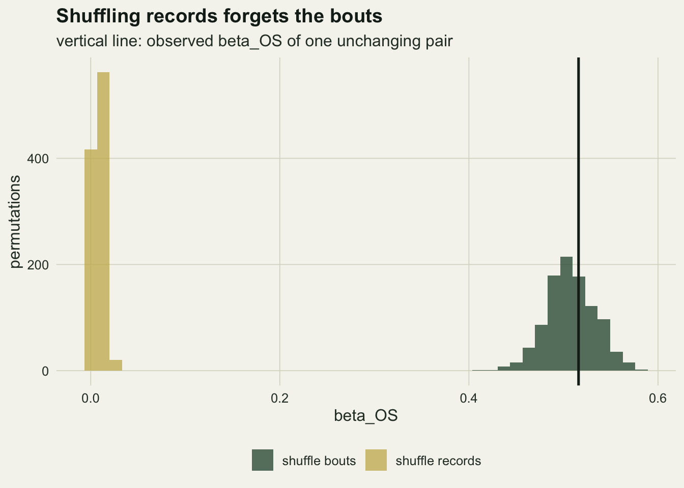

Figure 3: One pair of samples from an unchanging web, recorded in bouts of six visits: beta_OS against the null from shuffling records and the null from shuffling whole bouts.

When bout length changes between years

A cold, windy year gives shorter foraging bouts than a warm one, so the bout structure itself can differ between the years compared. The bout permutation keeps each year’s number of bouts and moves whole bouts, so after a shuffle both years hold a mixture of short and long bouts. Whether that matters depends on what a long bout adds. With full constancy a bout detects one link however long it is, so bout length cannot change the binary web, and bouts stay exchangeable. With partial constancy a long bout makes several plant choices, a short bout few, and under the null a long bout and a short bout are no longer draws from the same distribution. Shuffling them between years then changes how many plant choices each year holds.

Three designs share the webs, which do not change, and the two bout length distributions: in the short bout year a bout is one plus a Poisson count with mean 2 flower visits, in the long bout year one plus a Poisson count with mean 8. They differ only in how the 533 bouts are split between the years: 400 short and 133 long, which gives about 1200 records in each year; 267 of each; and 133 short with 400 long. One split alone cannot show which way the shuffle pushes, so three were run, and all three were fixed before the runs reported here.

A repair follows from the same argument. Bouts of the same length are exchangeable under the null whatever the constancy, so the shuffle can be restricted to bouts of equal length: within each length, the year labels are permuted, and each year keeps its exact count of bouts of every length. This stratified permutation is valid by construction; what it costs is information, because a length that occurs in only one year cannot be moved at all.

perm_strata <- function(bouts1, bouts2, nperm = n_perm) {
  obs  <- os_cells(bouts1, bouts2)
  pool <- rbind(bouts1, bouts2)
  lens <- rowSums(pool > 0)
  year <- rep(1:2, c(nrow(bouts1), nrow(bouts2)))
  base_order <- order(lens)
  null_os <- vapply(seq_len(nperm), function(i) {
    lab <- integer(length(year))
    lab[order(lens, runif(length(lens)))] <- year[base_order]
    os_cells(pool[lab == 1, , drop = FALSE], pool[lab == 2, , drop = FALSE])
  }, numeric(1))
  (1 + sum(null_os >= obs)) / (nperm + 1)
}
mu_short <- 2
mu_long  <- 8
varlen_cell <- function(n_short, n_long, constancy, rewire = 0, record_test = FALSE) {
  p_out <- replicate(n_test, {
    pr <- make_pair(0, rewire)
    b1 <- draw_bouts(pr$p1, n_short, 1 + rpois(n_short, mu_short), constancy)
    b2 <- draw_bouts(pr$p2, n_long, 1 + rpois(n_long, mu_long), constancy)
    width <- max(ncol(b1), ncol(b2))
    b1 <- pad_bouts(b1, width)
    b2 <- pad_bouts(b2, width)
    c(record = if (record_test) perm_records(b1[b1 > 0], b2[b2 > 0]) else NA,
      bout = perm_bouts(b1, b2), strata = perm_strata(b1, b2))
  })
  rowMeans(p_out <= 0.05)
}
# expected plant choices per year: a bout of length 1 + Poisson(mu) makes 1 + constancy * mu;
# after a bout shuffle both years draw from one pool, so their ratio is the ratio of bout counts
choice_ratio <- function(n_short, n_long, constancy) {
  c(observed = n_long * (1 + constancy * mu_long) / (n_short * (1 + constancy * mu_short)),
    shuffled = n_long / n_short)
}
set.seed(7702)
vl_a_c1  <- varlen_cell(400, 133, 1, record_test = TRUE)
vl_a_c05 <- varlen_cell(400, 133, 0.5, record_test = TRUE)
vl_b_c05 <- varlen_cell(267, 267, 0.5)
vl_b_c08 <- varlen_cell(267, 267, 0.8)
vl_c_c05 <- varlen_cell(133, 400, 0.5)
vl_pow_a_c1  <- varlen_cell(400, 133, 1, 0.3)
vl_pow_a_c05 <- varlen_cell(400, 133, 0.5, 0.3)
vl_pow_b_c05 <- varlen_cell(267, 267, 0.5, 0.3)
cr_a <- choice_ratio(400, 133, 0.5)
cr_b <- choice_ratio(267, 267, 0.5)
cr_c <- choice_ratio(133, 400, 0.5)
rbind(a_c1 = vl_a_c1, a_c05 = vl_a_c05, b_c05 = vl_b_c05, b_c08 = vl_b_c08, c_c05 = vl_c_c05,
      pow_a_c1 = vl_pow_a_c1, pow_a_c05 = vl_pow_a_c05, pow_b_c05 = vl_pow_b_c05)

          record  bout strata
a_c1           1 0.035  0.050
a_c05          1 0.000  0.065
b_c05         NA 0.775  0.060
b_c08         NA 0.255  0.075
c_c05         NA 1.000  0.055
pow_a_c1      NA 0.525  0.370
pow_a_c05     NA 0.110  0.615
pow_b_c05     NA 0.990  0.615

strata_size <- c(vl_a_c1[["strata"]], vl_a_c05[["strata"]], vl_b_c05[["strata"]],
                 vl_b_c08[["strata"]], vl_c_c05[["strata"]])
bout_size_pc <- c(vl_a_c05[["bout"]], vl_b_c05[["bout"]], vl_b_c08[["bout"]], vl_c_c05[["bout"]])
strata_z <- max(abs(strata_size - 0.05)) / mc_se_05
rbind(cr_a, cr_b, cr_c)

     observed shuffled
cr_a 0.831250 0.332500
cr_b 2.500000 1.000000
cr_c 7.518797 3.007519

With full constancy the bout permutation holds its level in the first split: it rejects in 0.035 of unchanging pairs, while the record permutation rejects in 1.000. With a constancy of one half the same split gives 0.000 for the bout permutation. Keep the bout lengths and change only the split, and it fails the other way. With 267 bouts in each year and a constancy of one half it rejects in 0.775 of unchanging pairs, at a constancy of 0.8 in 0.255, and with 133 short and 400 long bouts in 1.000. Under partial constancy the bout permutation is not a valid test when bout length differs between years: its false rejection rate ran from 0.000 to 1.000 in these runs, set by nothing more than how the bouts were split.

The expected number of plant choices shows why. A bout of length one plus a Poisson count with mean mu makes 1 + constancy times mu plant choices on average, so at a constancy of one half the long bout year holds 0.83 times the plant choices of the short bout year in the first split, 2.50 times in the second and 7.52 times in the third. After a bout shuffle both years draw from one pool, so the expected ratio becomes the ratio of bout counts: 0.33, 1.00 and 3.01. In the first split the shuffled years are more unequal in effort than the observed ones, their beta_OS runs higher, and the observed value looks ordinary. In the other two the shuffled years are more equal in effort than the observed ones, the null sits too low, and a plain difference in effort between the years is read as rewiring.

The stratified permutation holds its level in all five designs: its rejection rates on unchanging webs run from 0.050 to 0.075, and the largest departure from 0.05 is 1.6 Monte Carlo standard errors. Against rewiring in 30 per cent of pollinator species, at a constancy of one half, it rejects in 0.615 of pairs in the first split and 0.615 in the second. With full constancy, where the plain bout permutation is valid, the plain test is the stronger one, 0.525 against 0.370 for the stratified test, probably because a stratified shuffle cannot move bouts whose length occurs in one year only. The figure shows no power for the plain bout permutation where its size is wrong: with rewiring in the second split it rejected in 0.990 of pairs, against 0.775 with no rewiring at all, and that number describes the broken null, not the ability to detect rewiring.

size_df <- data.frame(
  scheme = rep(c("independent records, 500", "independent records, 3000",
                 "bouts of 6, constancy 1", "bouts of 6, constancy 0.5",
                 "400 short, 133 long, constancy 1", "400 short, 133 long, constancy 0.5",
                 "267 short, 267 long, constancy 0.5", "267 short, 267 long, constancy 0.8",
                 "133 short, 400 long, constancy 0.5"), each = 3),
  test = rep(c("shuffle records", "shuffle bouts", "shuffle bouts within length"), 9),
  reject = c(rpick(500, "unchanging"), NA, NA, rpick(3000, "unchanging"), NA, NA,
             bout_null_c1[["record"]], bout_null_c1[["bout"]], NA,
             bout_null_c05[["record"]], bout_null_c05[["bout"]], NA,
             vl_a_c1[c("record", "bout", "strata")], vl_a_c05[c("record", "bout", "strata")],
             vl_b_c05[c("record", "bout", "strata")], vl_b_c08[c("record", "bout", "strata")],
             vl_c_c05[c("record", "bout", "strata")]))
size_df <- size_df[!is.na(size_df$reject), ]
size_df$scheme <- factor(size_df$scheme, levels = rev(unique(size_df$scheme)))

pow_df <- data.frame(
  scheme = rep(c("independent records, 500: records", "independent records, 3000: records",
                 "bouts of 6, constancy 1: bouts"), each = 2),
  shift = rep(c("15 per cent of pollinators", "30 per cent of pollinators"), 3),
  reject = c(rpick(500, "rewiring 15 per cent"), rpick(500, "rewiring 30 per cent"),
             rpick(3000, "rewiring 15 per cent"), rpick(3000, "rewiring 30 per cent"),
             bout_rew15[["bout"]], bout_rew30[["bout"]]))
pow_df <- rbind(pow_df, data.frame(
  scheme = c("400 short, 133 long, constancy 1: bouts",
             "400 short, 133 long, constancy 1: within length",
             "400 short, 133 long, constancy 0.5: within length",
             "267 short, 267 long, constancy 0.5: within length"),
  shift = "30 per cent of pollinators",
  reject = c(vl_pow_a_c1[["bout"]], vl_pow_a_c1[["strata"]],
             vl_pow_a_c05[["strata"]], vl_pow_b_c05[["strata"]])))
pow_df$scheme <- factor(pow_df$scheme, levels = rev(unique(pow_df$scheme)))

p_size <- ggplot(size_df, aes(reject, scheme, colour = test)) +
  geom_vline(xintercept = 0.05, linetype = "dashed", colour = te_body, linewidth = 0.6) +
  geom_point(size = 3, alpha = 0.9) +
  scale_colour_manual(values = c(te_forest, te_gold, te_rust), name = NULL) +
  scale_x_continuous(limits = c(0, 1)) +
  guides(colour = guide_legend(nrow = 2)) +
  labs(x = "rejection rate, unchanging web", y = NULL, title = "Size") +
  theme_datasheet() +
  theme(legend.position = "bottom")
p_pow <- ggplot(pow_df, aes(reject, scheme, shape = shift)) +
  geom_point(size = 3, colour = te_ink, stroke = 1.1) +
  scale_shape_manual(values = c(1, 16), name = NULL) +
  scale_x_continuous(limits = c(0, 1)) +
  labs(x = "rejection rate, valid test", y = NULL, title = "Power") +
  theme_datasheet() +
  theme(legend.position = "bottom")
(p_size / p_pow) +
  plot_layout(heights = c(3.2, 2.5)) +
  plot_annotation(theme = theme_datasheet())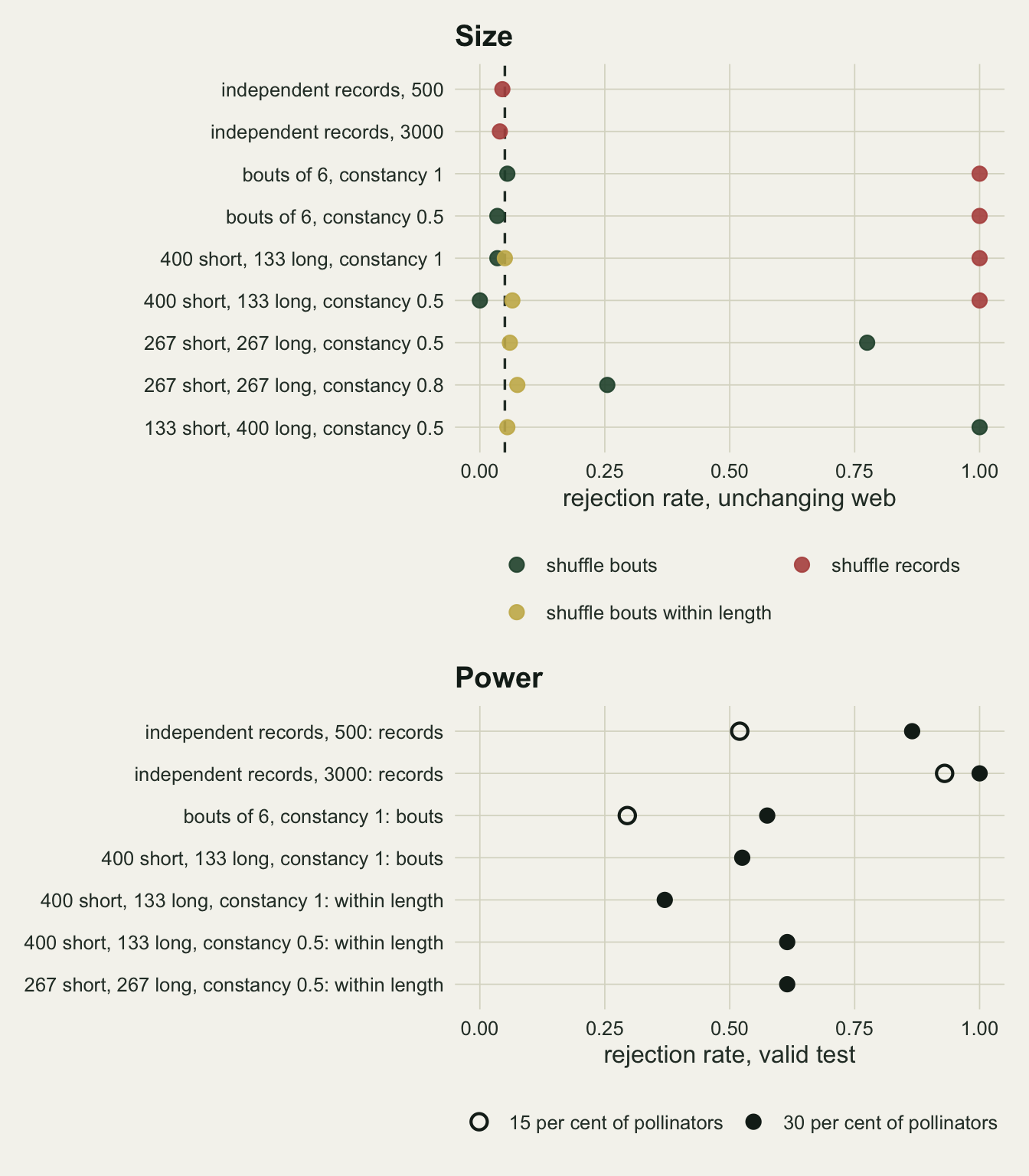

Figure 4: False rejection rates on unchanging webs for the record, bout and length-stratified bout permutations under each recording scheme, and power of the valid tests against rewiring.

What to report

Report the effort behind each web as the number of independent sampling units, not only the number of records, and say what a record is: a flower visit, a plant visit, or an insect caught on a transect. If records come in foraging bouts, the number of bouts is the effort that sets the floor.

Put the floor next to the partition. For each year the closed form needs only the estimated link probabilities and the effort, and a sample-level version comes for free from the permutation null. A rewiring component of 0.39 between two years of 500 independent records is what two samples of one unchanging web give on average; the same value between two years of 3000 records would be 2.0 times the floor at that effort.

If a share of turnover attributed to rewiring is reported, give the partition used and prefer the common denominator form, as Frund recommends, but do not read either share without the floor; Frund also argues that rewiring is poorly defined and that both forms can overstate it. Under pure species loss with no rewiring, the common denominator form still attributed 0.47 of the dissimilarity to rewiring at 3000 records.

Test rewiring with a permutation whose unit matches the way the data were collected, and say which unit was shuffled. Shuffling records when the records come in bouts produced false rejection rates of 1.00 in the simulation above. If bout length differs between years and flowers are not visited with full constancy, shuffle bouts only among bouts of the same length and report the bout length distribution of each year; a plain bout shuffle rejected unchanging webs in anything from 0.00 to 1.00 of pairs above.

Honest limits

The simulated web is a trait matching model with lognormal activity and no phenology. Real seasonal webs have species that do not overlap in time, and a year in which flowering shifts by two weeks changes which links can happen without any change in preference. CaraDonna and colleagues read part of that as rewiring; this post neither separates it nor tests it.

Rewiring was simulated as a new trait value for a fraction of pollinators, which moves those species to a new set of plants all at once. Rewiring in the sense of a gradual shift of visit frequencies among the same partners would be weaker in a binary web, and the power figures here should not be read as the power to detect it. The tests used only the binary form of beta_OS; quantitative versions weigh common links more and have a different floor, and Frund (2021) argues that both partitions can overstate rewiring in some respects, in particular for quantitative webs.

The closed form is a ratio of expectations and assumes the two samples are independent multinomial draws of fixed size. It does not include the restriction to species detected in both years, which is why it sits above the simulation at the lowest effort. For bout data, the same formula applies with bouts as the effort only under full constancy; with partial constancy the detection probability of a link per bout has no simple form and would have to be simulated.

The permutation tests assume that the two years are exchangeable under the null at the level of the unit shuffled. That rules out a real change in species activity between years that is not rewiring, for example a pollinator that is twice as common in the second year: its links are detected more often, beta_OS can rise, and a permutation of records or bouts will call that a difference between webs, which it is, but not a change of partners. Species loss did not raise the rejection rate here, where the lost species were removed outright rather than thinned. The bout generator used a fixed number of bouts per year and bouts that are independent of each other; bouts by the same individual across a day, or several bees sharing a patch, are a further level of dependence that a bout permutation does not handle, and shuffling at the level of census walks or days would be the next step. The length stratified shuffle assumes that bouts of equal length are exchangeable, which fails if constancy itself differs between years; the strata would then have to carry that difference too, and each extra stratum removes information. Its power also depends on how far the bout length distributions of the two years overlap, and it was run here on one pair of Poisson length distributions.

The floor, the shares and the test results are for a web of 25 plants and 40 pollinators. By the closed form, a larger web with more rare links has a higher floor at the same effort, and the effort needed to reach a given floor grows with it.

References

Poisot T, Canard E, Mouillot D, Mouquet N, Gravel D 2012 Ecology Letters 15(12):1353-1361 (10.1111/ele.12002)

Frund J 2021 Ecosphere 12(7):e03653 (10.1002/ecs2.3653)

Frund J, McCann KS, Williams NM 2016 Oikos 125(4):502-513 (10.1111/oik.02256)

CaraDonna PJ, Petry WK, Brennan RM, Cunningham JL, Bronstein JL, Waser NM, Sanders NJ 2017 Ecology Letters 20(3):385-394 (10.1111/ele.12740)

Related tutorials

• Checking a network analysis
• Null models for interaction networks
• Permutation tests for social networks
• Bipartite network metrics from scratch