Null models for interaction networks

Why a network metric means nothing on its own: three nulls (equiprobable, proportional, fixed-fixed), a nestedness verdict that flips with the null, and the robustness of a web to species loss, all in base R.

The earlier posts on network metrics and modularity ended on the same warning: a raw number cannot be read on its own, because a structureless web still returns a positive connectance, nestedness or modularity. The fix is a null model, a way of shuffling the web to ask what its value would be by chance. The catch is that there is more than one way to shuffle, and the verdict can flip depending on which one you pick. This post codes three nulls, shows a nestedness result changing from decisive to non-significant across them, and then applies the same logic to how robust a web is to species loss. All of it is base R, including the Patefield algorithm, which ships as r2dtable.

A web nested by its degree distribution

The test web is deliberately plain: interaction probability is the product of a pollinator’s activity and a plant’s activity, with no extra structure layered on. Heterogeneous activity alone makes the matrix look nested, because busy species interact with many partners and the quiet ones interact with subsets of those.

set.seed(4262)
A0 <- 16L; P0 <- 14L
a_row <- exp(rnorm(A0, 0, 0.9)); b_col <- exp(rnorm(P0, 0, 0.8))
Pr <- outer(a_row, b_col); Pr <- Pr / max(Pr)
B <- matrix(rbinom(A0 * P0, 1, 0.85 * Pr), A0, P0)
B[cbind(seq_len(A0), max.col(Pr))] <- 1
B[cbind(max.col(t(Pr)), seq_len(P0))] <- 1
B <- B[rowSums(B) > 0, colSums(B) > 0, drop = FALSE]
A <- nrow(B); P <- ncol(B); L <- sum(B)
NODF_obs <- nodf(B)
c(pollinators = A, plants = P, links = L, connectance = round(L / (A * P), 3), NODF = round(NODF_obs, 2))

pollinators      plants       links connectance        NODF 
     16.000      14.000      44.000       0.196      66.430 

The web has 16 pollinators, 14 plants, connectance 0.20 and an observed nestedness of NODF = 66.4. On its own that number says nothing. The question is what a random web would give.

Three ways to shuffle

Each null keeps some feature of the observed web and randomises the rest, and they differ in how much they keep.

The equiprobable null keeps only the number of links: it scatters the same count of interactions across the matrix with every cell equally likely. The proportional null, in the spirit of Vazquez and Aizen (2003), keeps the marginal activity: a cell’s chance of being filled rises with the product of its row and column degree, so busy species stay busy on average. The fixed-fixed null keeps both degree sequences exactly: every species ends with the same number of partners it started with, only rewired. The last is the strict test, generated by swapping checkerboard pairs that leave every row and column total untouched.

null_equi <- function() { z <- numeric(A * P); z[sample(A * P, L)] <- 1; matrix(z, A, P) }
rd0 <- rowSums(B); cd0 <- colSums(B)
Pp <- outer(rd0, cd0); Pp <- pmin(Pp / sum(Pp) * L, 1)
null_prop <- function() matrix(rbinom(A * P, 1, Pp), A, P)
null_swap <- function(M, nsw = 3000) {
  for (s in seq_len(nsw)) {
    ii <- sample(nrow(M), 2); jj <- sample(ncol(M), 2); sub <- M[ii, jj]
    if (all(sub == matrix(c(1, 0, 0, 1), 2)))      M[ii, jj] <- matrix(c(0, 1, 1, 0), 2)
    else if (all(sub == matrix(c(0, 1, 1, 0), 2))) M[ii, jj] <- matrix(c(1, 0, 0, 1), 2)
  }
  M
}
nrep <- 299L
set.seed(11); N_equi <- replicate(nrep, nodf(null_equi()))
set.seed(12); N_prop <- replicate(nrep, nodf(null_prop()))
set.seed(13); N_swap <- replicate(nrep, nodf(null_swap(B)))
zscore <- function(obs, nd) (obs - mean(nd)) / sd(nd)
pval   <- function(obs, nd) (1 + sum(nd >= obs)) / (length(nd) + 1)

The verdict flips

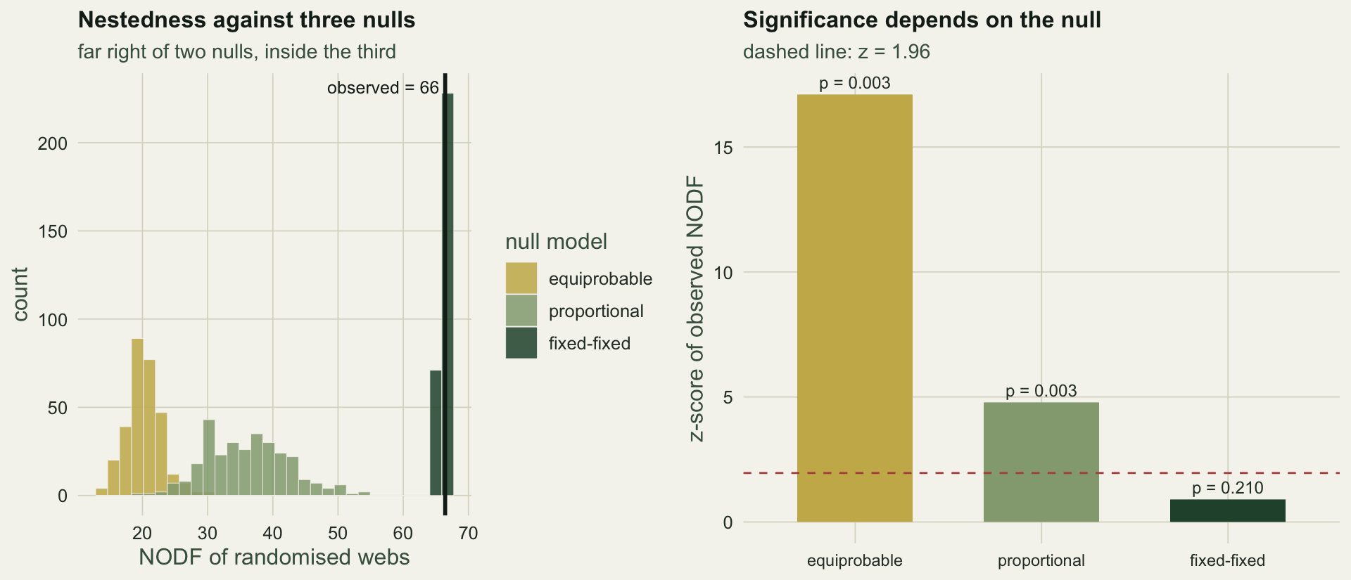
Reading the observed NODF against each null gives three different answers.

verdict <- data.frame(
  null = c("equiprobable", "proportional", "fixed-fixed"),
  null_mean = c(mean(N_equi), mean(N_prop), mean(N_swap)),
  z = c(zscore(NODF_obs, N_equi), zscore(NODF_obs, N_prop), zscore(NODF_obs, N_swap)),
  p = c(pval(NODF_obs, N_equi), pval(NODF_obs, N_prop), pval(NODF_obs, N_swap)))
z_equi <- verdict$z[1]; z_prop <- verdict$z[2]; z_swap <- verdict$z[3]
p_swap <- verdict$p[3]
round(verdict[, -1], 3)

  null_mean      z     p
1    20.263 17.095 0.003
2    36.083  4.780 0.003
3    66.138  0.895 0.210

Against the equiprobable null the web is overwhelmingly nested, with a z-score of 17.1. Against the proportional null it is still clearly nested, z = 4.8. Against the fixed-fixed null it is not nested at all: z = 0.9 and p = 0.21. The observed NODF of 66.4 sits almost exactly on the fixed-fixed null mean of 66.1, because once the degree sequence is fixed the nestedness is nearly pinned. The reading is the standard one (Ulrich, Almeida-Neto and Gotelli 2009): this web is no more nested than its degree distribution forces it to be, and the dramatic result under the looser nulls came from the activity heterogeneity, not from any extra nested arrangement.

Figure 1: Left: the distribution of NODF under each null, with the observed value marked. Right: the z-score of the observed NODF against each null; the dashed line is the two-sided five per cent threshold.

Robustness to species loss

The same logic runs through a different question: how well does the web hold together as species disappear? A common measure removes plants one at a time and counts the pollinators that lose every partner and go secondarily extinct (Memmott et al 2004). The attack-tolerance curve plots the fraction of pollinators still surviving against the fraction of plants removed, and the robustness R is the area under it (Burgos et al 2007): near one if pollinators persist until almost every plant is gone, near zero if the web collapses early.

survival_curve <- function(M, order_cols) {
  removed <- logical(ncol(M)); surv <- numeric(ncol(M) + 1); surv[1] <- 1
  for (k in seq_along(order_cols)) {
    removed[order_cols[k]] <- TRUE
    surv[k + 1] <- mean(rowSums(M[, !removed, drop = FALSE]) > 0)
  }
  surv
}
robustness_R <- function(surv) { x <- seq(0, 1, length.out = length(surv)); sum((surv[-1] + surv[-length(surv)]) / 2 * diff(x)) }
deg_c <- colSums(B)
surv_most  <- survival_curve(B, order(deg_c, decreasing = TRUE))
surv_least <- survival_curve(B, order(deg_c, decreasing = FALSE))
set.seed(1); surv_rand <- survival_curve(B, sample(P))
R_most <- robustness_R(surv_most); R_least <- robustness_R(surv_least)
set.seed(7); R_rand <- mean(replicate(200, robustness_R(survival_curve(B, sample(P)))))
c(most_connected = round(R_most, 3), random = round(R_rand, 3), least_connected = round(R_least, 3))

 most_connected          random least_connected 
          0.299           0.653           0.964 

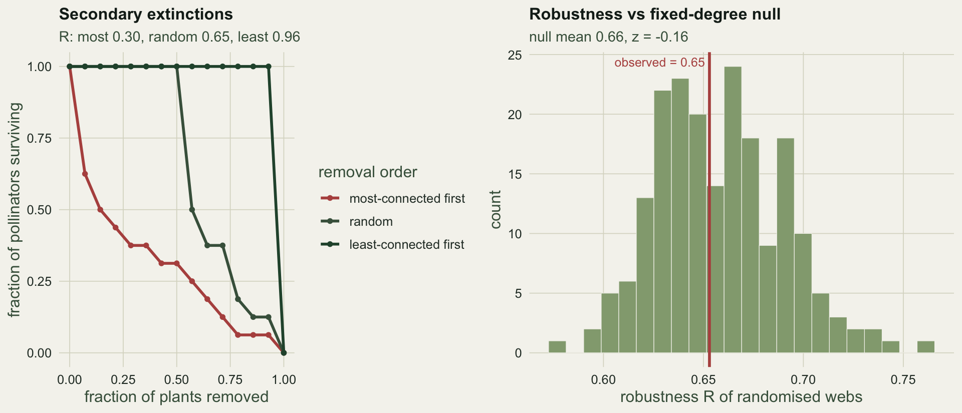
The order of loss dominates the answer. Removing the best-connected plants first collapses the web fast, giving R = 0.30; removing the least-connected first barely touches the pollinators, R = 0.96; a random order sits between at 0.65. A single robustness figure is meaningless without saying which extinction order it assumes, just as a single NODF is meaningless without a null.

And robustness itself needs a null. Is this web more or less robust than a random web with the same degree sequence?

set.seed(21)
R_null <- replicate(199, {
  M <- null_swap(B)
  mean(replicate(30, robustness_R(survival_curve(M, sample(ncol(M))))))
})
z_R <- zscore(R_rand, R_null)
c(null_mean = round(mean(R_null), 3), null_sd = round(sd(R_null), 3),
  observed = round(R_rand, 3), z = round(z_R, 2))

null_mean   null_sd  observed         z 
    0.658     0.032     0.653    -0.160 

The observed random-order robustness of 0.65 sits right on the null mean of 0.66, z = -0.16. The web is exactly as robust as its degree sequence implies, no more and no less. As with nestedness, the interesting quantity is the departure from a null, and here there is none.

Figure 2: Left: attack-tolerance curves for three removal orders, with the robustness R of each. Right: the observed random-order robustness against the fixed-degree null distribution.

Where this leaves you

A network metric is a comparison waiting for a baseline. The equiprobable null asks whether the web has any structure at all, the proportional null whether it has structure beyond the activity of its species, and the fixed-fixed null whether it has structure beyond the full degree sequence. They are different questions, and here they gave nestedness answers ranging from decisive to null. The robustness of the web behaves the same way: it depends on the assumed order of loss and, measured against a null, adds nothing to what the degree sequence already sets. Choosing the null is choosing the question, and the last post, checking a network analysis, turns to a confound that no null repairs: how hard the web was sampled.

References

Bascompte, J., Jordano, P., Melian, C. J. and Olesen, J. M. (2003). The nested assembly of plant-animal mutualistic networks. Proceedings of the National Academy of Sciences, 100(16), 9383-9387. https://doi.org/10.1073/pnas.1633576100

Burgos, E., Ceva, H., Perazzo, R. P. J., Devoto, M., Medan, D., Zimmermann, M. and Delbue, A. M. (2007). Why nestedness in mutualistic networks? Journal of Theoretical Biology, 249(2), 307-313. https://doi.org/10.1016/j.jtbi.2007.07.030

Memmott, J., Waser, N. M. and Price, M. V. (2004). Tolerance of pollination networks to species extinctions. Proceedings of the Royal Society B: Biological Sciences, 271(1557), 2605-2611. https://doi.org/10.1098/rspb.2004.2909

Patefield, W. M. (1981). Algorithm AS 159: an efficient method of generating random R x C tables with given row and column totals. Journal of the Royal Statistical Society. Series C (Applied Statistics), 30(1), 91-97. https://doi.org/10.2307/2346669

Ulrich, W., Almeida-Neto, M. and Gotelli, N. J. (2009). A consumer’s guide to nestedness analysis. Oikos, 118(1), 3-17. https://doi.org/10.1111/j.1600-0706.2008.17053.x

Vazquez, D. P. and Aizen, M. A. (2003). Null model analyses of specialization in plant-pollinator interactions. Ecology, 84(9), 2493-2501. https://doi.org/10.1890/02-0587

Related tutorials

• Bipartite network metrics from scratch
• Modularity in ecological networks
• Nestedness and the NODF metric
• Checking a network analysis