Checking a network analysis

How far sampling effort, network size and unseen links move connectance, H2’ and nestedness, what a null model rescues, and the one thing the matrix can never tell you.

The three earlier posts in this series built the toolkit: metrics for describing a web, modularity for its compartments, and null models for deciding whether any of it beats chance. Each ended on the same unfinished thought: the numbers move when the sampling moves. This post makes that concrete by building a web whose true interaction probabilities are known, then sampling it at different intensities and watching what happens. Some of the damage a null model repairs. One part of it nothing repairs, and that is the honest limit worth carrying into your own data.

A web whose truth you know

Every interaction matrix in the wild is a sample: the observer watched for a fixed number of hours and wrote down what happened. To see what that sampling does, define the true interaction probabilities first, then draw from them.

set.seed(4263)
A <- 20L; P <- 16L
a_row <- exp(rnorm(A, 0, 0.8)); b_col <- exp(rnorm(P, 0, 0.7))
mu <- runif(A); pos <- seq(0.05, 0.95, length.out = P); niche_w <- 0.22
Ptrue <- outer(a_row, b_col) * exp(-(outer(mu, pos, "-")^2) / (2 * niche_w^2))
Ptrue <- Ptrue / sum(Ptrue)
n_possible <- sum(Ptrue > 1e-6)
c(cells = A * P, ecologically_possible = n_possible)

                cells ecologically_possible 
                  320                   315 

Of the 320 cells, 315 carry a non-negligible probability: those are the links that exist in this system. The rest are trait mismatches that will never be observed no matter how long you watch. Sampling n interactions is a multinomial draw over the cells.

The first diagnostic: how much of the web have you seen?

Before any index, ask how complete the sample is. The interaction accumulation curve counts distinct links discovered as interactions are recorded, the network analogue of a species accumulation curve. A curve still climbing at the end of the data is a web with links left to find.

set.seed(6)
pool <- sample(rep(seq_len(A * P), round(Ptrue * 100000)))
grid_n <- c(seq(20, 400, 20), seq(500, 3000, 250))
accum <- vapply(grid_n, function(k) length(unique(pool[seq_len(k)])), numeric(1))
acc_df <- data.frame(sampled = grid_n, unique_links = accum)
acc_end <- accum[length(accum)]
c(links_found_at_3000 = acc_end, links_that_exist = n_possible,
  fraction = round(acc_end / n_possible, 2))

links_found_at_3000    links_that_exist            fraction 
             244.00              315.00                0.77 

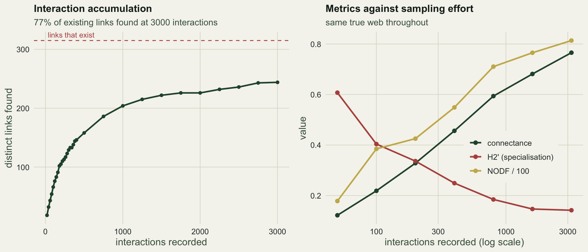
After 3000 recorded interactions the curve has found 244 of the 315 links that exist, 77 per cent, and is still rising. Real pollination datasets are usually far short of that (Chacoff et al 2012; Jordano 2016), which matters because the missing links are not a random subset: they are the rare ones.

Every metric drifts with effort

Now sample the same true web at increasing intensity and recompute the indices from the earlier posts.

samp_metrics <- function(n) {
  W <- matrix(rmultinom(1, n, as.vector(Ptrue)), A, P)
  Wt <- W[rowSums(W) > 0, colSums(W) > 0, drop = FALSE]
  c(effort = n, connectance = sum(W > 0) / (A * P),
    H2prime = H2prime(Wt), NODF = nodf((Wt > 0) * 1))
}
set.seed(5)
efforts <- c(50, 100, 200, 400, 800, 1600, 3200)
drift <- as.data.frame(t(vapply(efforts, samp_metrics, numeric(4))))
conn_lo <- drift$connectance[1]; conn_hi <- drift$connectance[nrow(drift)]
h2_lo <- drift$H2prime[1]; h2_hi <- drift$H2prime[nrow(drift)]
nodf_lo <- drift$NODF[1]; nodf_hi <- drift$NODF[nrow(drift)]
round(drift, 3)

  effort connectance H2prime   NODF
1     50       0.122   0.607 17.820
2    100       0.219   0.404 38.474
3    200       0.328   0.336 42.527
4    400       0.456   0.249 54.896
5    800       0.594   0.185 71.032
6   1600       0.681   0.147 76.533
7   3200       0.766   0.142 81.365

Nothing about the ecology changed between these rows. Only the watching did, and every number moved a long way. Connectance climbed from 0.12 to 0.77, because more effort finds more rare links. Nestedness rose from 18 to 81. Most striking, the specialisation index H2’ fell from 0.61 to 0.14: at low effort the web looks highly specialised, and the apparent specialisation dissolves as sampling improves. H2’ was introduced in the first post as the index that travels best because it standardises against the marginal totals. It still drifts by a factor of four here. A thin sample makes generalists look like specialists, which is the same confound that made poorly sampled pollinators score high on d’ (Bluthgen et al 2008; Frund et al 2016).

Figure 1: Left: the interaction accumulation curve, still climbing after 3000 recorded interactions. Right: connectance, H2’ and nestedness against sampling effort on a log scale; all three drift steadily although the underlying web never changes.

Size dependence: bigger webs look sparser

The second confound is dimension. Generate webs from the same process at different species richness, with effort scaled to richness so that per-species sampling is constant.

gen_web <- function(S, eff_per_sp = 32) {
  a <- exp(rnorm(S, 0, 0.7)); b <- exp(rnorm(S, 0, 0.6))
  mu_s <- runif(S); pos_s <- seq(0.05, 0.95, length.out = S)
  Pt <- outer(a, b) * exp(-(outer(mu_s, pos_s, "-")^2) / (2 * 0.22^2)); Pt <- Pt / sum(Pt)
  W <- matrix(rmultinom(1, eff_per_sp * S, as.vector(Pt)), S, S)
  W[rowSums(W) > 0, colSums(W) > 0, drop = FALSE]
}
set.seed(77)
sizes <- c(6, 9, 12, 15, 18, 21, 24)
size_res <- as.data.frame(t(vapply(sizes, function(S) {
  reps <- replicate(8, { W <- gen_web(S); c(conn = sum(W > 0) / (nrow(W) * ncol(W)), nd = nodf((W > 0) * 1)) })
  c(size = S, connectance = mean(reps["conn", ]), NODF = mean(reps["nd", ]))
}, numeric(3))))
size_conn_lo <- size_res$connectance[nrow(size_res)]; size_conn_hi <- size_res$connectance[1]
round(size_res, 3)

  size connectance   NODF
1    6       0.733 67.181
2    9       0.657 67.755
3   12       0.582 65.539
4   15       0.577 64.056
5   18       0.554 63.599
6   21       0.516 62.539
7   24       0.473 59.972

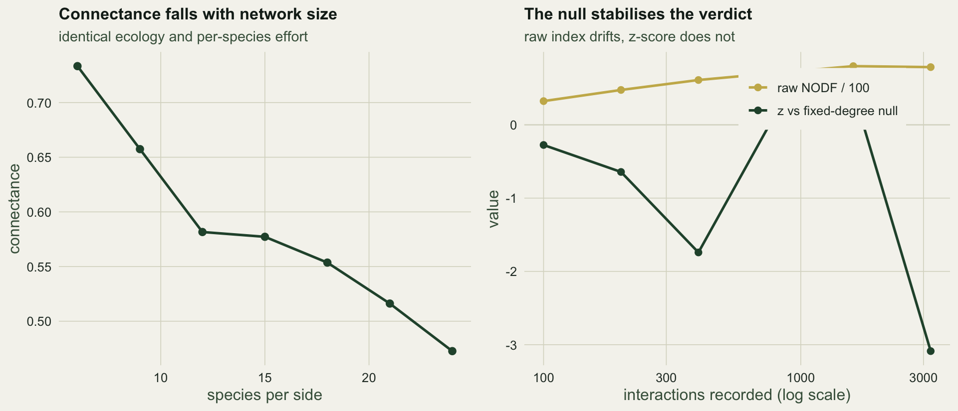
The niche width, the abundance spread and the effort per species are identical across these webs. Only the number of species differs, and connectance falls from 0.73 in the smallest web to 0.47 in the largest. This is the well-known scaling of connectance with richness (Olesen and Jordano 2002; Bluthgen 2010): a species cannot double its partners just because the web doubled in size, so the realised fraction of possible cells shrinks. Comparing raw connectance between a 20-species web and a 60-species web says more about their dimensions than their ecology.

What the null model rescues

Given that the raw numbers move, does the null-model machinery from the previous post fare better? Recompute nestedness across effort, but read each value against a fixed-degree null rather than on its own.

set.seed(41)
zt <- as.data.frame(t(vapply(c(100, 200, 400, 800, 1600, 3200), function(n) {
  W <- matrix(rmultinom(1, n, as.vector(Ptrue)), A, P)
  B <- (W > 0) * 1; B <- B[rowSums(B) > 0, colSums(B) > 0, drop = FALSE]
  obs <- nodf(B); nd <- replicate(99, nodf(null_swap(B)))
  c(effort = n, raw_NODF = obs, z = (obs - mean(nd)) / sd(nd))
}, numeric(3))))
z_raw_lo <- zt$raw_NODF[1]; z_raw_hi <- zt$raw_NODF[nrow(zt)]
z_range <- range(zt$z)
round(zt, 2)

  effort raw_NODF     z
1    100    32.35 -0.27
2    200    47.59 -0.64
3    400    61.14 -1.74
4    800    70.80  0.16
5   1600    80.09  0.46
6   3200    78.74 -3.09

The raw nestedness climbs from 32 to 79 across this range of effort, a factor of 2.4. The z-score does not follow it: it wanders between -3.1 and 0.5 with no systematic trend, and never gives a convincing signal. That is the right answer, because this web was built with no nestedness beyond what its degree sequence forces. The null does its job: the verdict is stable even while the raw index quadruples. This is the practical case for reporting departures from a null rather than raw values, and it holds for modularity and specialisation as much as nestedness.

The z-score is noisy, though, and reading a single one as a precise effect size would overstate it. It answers a yes or no question about structure beyond the degrees; it does not restore the raw metric’s comparability.

Figure 2: Left: connectance against species richness, with per-species effort held constant. Right: raw nestedness rises steeply with effort while its z-score against a fixed-degree null shows no systematic drift.

The honest limit: a zero has two meanings

Here is what no null model, no standardised index and no amount of care with the analysis can fix. Take a realistic sample and look at the empty cells.

set.seed(42)
W_obs <- matrix(rmultinom(1, 600, as.vector(Ptrue)), A, P)
zero_cells <- which(W_obs == 0)
thr <- 1e-4
n_forbidden <- sum(Ptrue[zero_cells] < thr)
n_missing   <- sum(Ptrue[zero_cells] >= thr)
exp_visits  <- 600 * Ptrue[zero_cells][Ptrue[zero_cells] >= thr]
c(zeros = length(zero_cells), forbidden = n_forbidden, missing = n_missing,
  pct_missing = round(100 * n_missing / length(zero_cells)),
  median_expected_visits = round(median(exp_visits), 2))

                 zeros              forbidden                missing 
                149.00                  55.00                  94.00 
           pct_missing median_expected_visits 
                 63.00                   0.36 

The sample has 149 empty cells. Of those, 55 are genuine: trait mismatches, phenological non-overlap, links that cannot happen. The other 94, which is 63 per cent of the zeros, are real interactions that simply were not seen, most of them expected to occur less than once at this effort (median 0.36 expected visits). In the matrix these two kinds of zero are the same character. Nothing in the data distinguishes a forbidden link from a missing one, and yet every index in this series treats them identically: connectance counts them as absences, NODF reads them as gaps in a nested pattern, H2’ scores them as evidence of choosiness.

Only outside information separates them. Trait measurements can rule a link impossible, phenological records can show two species never overlap, and more effort turns a missing link into an observed one (Olesen et al 2011; Jordano 2016). None of it comes from the matrix. This is the same shape as the honest limits elsewhere on this blog: the unseen species behind a richness estimate, the untestable exchangeability behind a conformal interval, the assumption of no unmeasured confounding behind a causal claim. The checking constrains the reading; it does not license certainty.

Where this leaves you

Three checks are worth running on any interaction network before the indices are reported. Plot the interaction accumulation curve and say plainly how complete the sample is. Refuse to compare raw connectance, linkage density or nestedness across webs of different size or effort, because those numbers scale with both. Report departures from an explicit null instead of raw values, since the z-score survives a fourfold drift in the raw index that would otherwise be read as ecology.

None of that reaches the deepest problem. Most of the zeros in a typical web are links that exist and were missed, and the matrix cannot tell you which. Network analysis is a description of a sample, and the further your conclusions travel from that sample, the more they lean on evidence that is not in it.

References

Bluthgen, N. (2010). Why network analysis is often disconnected from community ecology: a critique and an ecologist’s guide. Basic and Applied Ecology, 11(3), 185-195. https://doi.org/10.1016/j.baae.2010.01.001

Bluthgen, N., Frund, J., Vazquez, D. P. and Menzel, F. (2008). What do interaction network metrics tell us about specialization and biological traits? Ecology, 89(12), 3387-3399. https://doi.org/10.1890/07-2121.1

Chacoff, N. P., Vazquez, D. P., Lomascolo, S. B., Stevani, E. L., Dorado, J. and Padron, B. (2012). Evaluating sampling completeness in a desert plant-pollinator network. Journal of Animal Ecology, 81(1), 190-200. https://doi.org/10.1111/j.1365-2656.2011.01883.x

Frund, J., McCann, K. S. and Williams, N. M. (2016). Sampling bias is a challenge for quantifying specialization and network structure: lessons from a quantitative niche model. Oikos, 125(4), 502-513. https://doi.org/10.1111/oik.02256

Jordano, P. (2016). Sampling networks of ecological interactions. Functional Ecology, 30(12), 1883-1893. https://doi.org/10.1111/1365-2435.12763

Olesen, J. M. and Jordano, P. (2002). Geographic patterns in plant-pollinator mutualistic networks. Ecology, 83(9), 2416-2424.

Olesen, J. M., Bascompte, J., Dupont, Y. L., Elberling, H., Rasmussen, C. and Jordano, P. (2011). Missing and forbidden links in mutualistic networks. Proceedings of the Royal Society B: Biological Sciences, 278(1706), 725-732. https://doi.org/10.1098/rspb.2010.1371

Related tutorials

• Bipartite network metrics from scratch
• Null models for interaction networks
• Modularity in ecological networks
• Rarefaction and accumulation curves

## References

Bluthgen N 2010 Basic and Applied Ecology 11(3):185-195 (10.1016/j.baae.2010.01.001)
Bluthgen N, Frund J, Vazquez DP, Menzel F 2008 Ecology 89(12):3387-3399 (10.1890/07-2121.1)