---
title: "Bipartite network metrics from scratch"
description: "Connectance, generality, vulnerability and the specialisation indices H2' and d' for a plant-pollinator web, in base R, with the sampling caveats spelled out."
date: "2026-06-09 13:00"
date-modified: "2026-09-30"
categories: [R, ecological networks, species interactions, ggplot2, ecology tutorial]
image: thumbnail.png
image-alt: "Heatmap of a plant-pollinator interaction matrix, twelve rows by ten columns, mostly pale with two much darker green cells marking the heaviest pairings."
---
*Corrected 30 September 2026: d' was rescaled by one constant for every pollinator, the divergence for putting all visits on the rarest plant, which is out of reach for most of them and overstated how strongly d' tracks sampling depth in this web; it is now rescaled by each species' own ceiling, as Bluthgen and colleagues define it, and the sampling section reports the weaker trend that follows.*
A plant-pollinator dataset, a host-parasite rearing table or a seed-disperser log all share a shape: a rectangular matrix where rows are one set of species, columns are another, and each cell counts the interactions between a pair. A handful of numbers are then meant to summarise the whole web: how connected it is, how specialised the species are, whether a few players carry most of the links. This post codes those descriptors by hand, so the definitions stay visible, and it flags the two properties that make raw network numbers hard to compare: they depend on the size of the matrix and on how hard the web was sampled.
The reference implementation for all of this is the `bipartite` package (Dormann et al 2009); here the render path is base R only, which keeps every index a few lines of readable code.
```{r}
#| label: setup
#| echo: false
#| message: false
#| warning: false
library(ggplot2)
library(grid)
te_ink <- "#16241d"; te_body <- "#2c3a31"; te_forest <- "#275139"; te_label <- "#46604a"
te_sage <- "#93a87f"; te_paper <- "#f5f4ee"; te_line <- "#dad9ca"; te_gold <- "#c9b458"
theme_te <- function(base = 12) theme_minimal(base_size = base) +
theme(plot.background = element_rect(fill = te_paper, colour = NA),
panel.background = element_rect(fill = te_paper, colour = NA),
panel.grid.minor = element_blank(),
panel.grid.major = element_line(colour = te_line, linewidth = 0.3),
axis.text = element_text(colour = te_body), axis.title = element_text(colour = te_label),
plot.title = element_text(colour = te_ink, face = "bold", size = rel(1.02)),
plot.subtitle = element_text(colour = te_label, size = rel(0.9)),
legend.text = element_text(colour = te_body), legend.title = element_text(colour = te_label))
```
## A synthetic plant-pollinator web
The matrix comes from a simple model: each pollinator has an abundance and a niche position, each plant a position on the same axis, and the expected number of visits falls off with the distance between them. Poisson counts finish it off.
```{r}
#| label: build-web
set.seed(4260)
A0 <- 12L; P0 <- 10L
poll_ab   <- exp(rnorm(A0, 0, 0.7))
plant_ab  <- exp(rnorm(P0, 0, 0.6))
poll_mu   <- runif(A0, 0, 1)
plant_pos <- seq(0.05, 0.95, length.out = P0)
niche_w   <- 0.18
lam <- outer(poll_ab, plant_ab) * exp(-(outer(poll_mu, plant_pos, "-")^2) / (2 * niche_w^2))
lam <- lam / sum(lam) * 600
W <- matrix(rpois(A0 * P0, lam), A0, P0)
rownames(W) <- paste0("poll", seq_len(A0)); colnames(W) <- paste0("plant", seq_len(P0))
W <- W[rowSums(W) > 0, colSums(W) > 0, drop = FALSE]
A <- nrow(W); P <- ncol(W)
m <- sum(W); rs <- rowSums(W); cs <- colSums(W)
c(pollinators = A, plants = P, interactions = m)
```
The web has `r A` pollinators, `r P` plants and `r m` recorded interactions.
## Connectance and links: the descriptors that scale with size
The most basic number is **connectance**: the fraction of possible links that are realised. With `A` rows and `P` columns there are `A * P` possible cells, and connectance is the count of non-empty cells divided by that.
```{r}
#| label: connectance
n_links   <- sum(W > 0)
connect   <- n_links / (A * P)
links_per <- n_links / (A + P)
c(links = n_links, connectance = round(connect, 3), links_per_species = round(links_per, 2))
```
Here `r n_links` of the `r A * P` cells are filled, so connectance is `r sprintf("%.3f", connect)` and there are `r sprintf("%.2f", links_per)` links per species. These are honest counts, but they are the wrong things to compare across studies. Connectance falls as a web grows, because the number of possible cells grows faster than the number a species can plausibly use, and it climbs when a web is sampled harder, because more rare links get recorded. Two webs with identical ecology but different dimensions or effort will report different connectance. The indices below are built to lean on this less.
## Quantitative descriptors: effective partners
A pollinator that splits its visits evenly across five plants is more of a generalist than one that makes ninety per cent of its visits to a single plant, even if both touch five plants. The **effective number of partners** captures that by exponentiating the Shannon diversity of a species' interactions.
```{r}
#| label: effective-partners
shannon_eff <- function(x) { p <- x[x > 0] / sum(x); exp(-sum(p * log(p))) }
eff_plants <- apply(W, 1, shannon_eff)   # effective plants per pollinator
eff_polls  <- apply(W, 2, shannon_eff)   # effective pollinators per plant
generality   <- sum((rs / m) * eff_plants)
vulnerability<- sum((cs / m) * eff_polls)
link_density <- (generality + vulnerability) / 2
w_connect    <- link_density / (A + P)
round(c(generality, vulnerability, link_density, w_connect), 3)
```
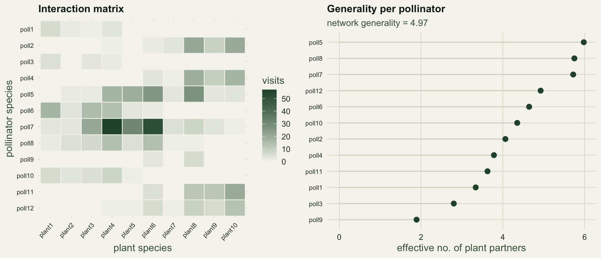
Averaging these effective counts across species, weighted by how many interactions each carries, gives the quantitative descriptors of Bersier et al (2002): **generality** `r sprintf("%.2f", generality)` (the effective plants an average pollinator uses), **vulnerability** `r sprintf("%.2f", vulnerability)` (the effective pollinators an average plant receives), their mean the weighted **linkage density** `r sprintf("%.2f", link_density)`, and the weighted connectance `r sprintf("%.3f", w_connect)`. Because they count effective rather than raw partners, a single stray visit barely moves them, unlike the binary link count.
## Network specialisation: H2'
The index that travels best across webs is **H2'** (Bluthgen et al 2006). It asks how far the observed spread of interactions departs from what the row and column totals alone would produce. Write every cell as a proportion of the grand total and take the two-dimensional Shannon entropy H2. The most even web consistent with the same marginal totals is the one where interactions are independent of identity, and its entropy is just the sum of the marginal entropies; the least even is the most tightly packed web with those totals. H2' rescales the observed entropy between the two.
```{r}
#| label: h2prime
pmat  <- W[W > 0] / m
H2    <- -sum(pmat * log(pmat))
r <- rs / m; cc <- cs / m
H2max <- -sum(r[r > 0] * log(r[r > 0])) - sum(cc[cc > 0] * log(cc[cc > 0]))
# least-even coupling with the same marginals: greedily pack the largest feasible cell
pack_entropy <- function(rw, cl, tot) {
  ent <- 0
  repeat {
    if (sum(rw) <= 0) break
    best <- -1; bi <- bj <- NA
    for (i in which(rw > 0)) for (j in which(cl > 0)) {
      v <- min(rw[i], cl[j]); if (v > best) { best <- v; bi <- i; bj <- j }
    }
    p <- best / tot; ent <- ent - p * log(p)
    rw[bi] <- rw[bi] - best; cl[bj] <- cl[bj] - best
  }
  ent
}
H2min   <- pack_entropy(rs, cs, m)
H2prime <- (H2max - H2) / (H2max - H2min)
round(c(H2 = H2, H2max = H2max, H2min = H2min, H2prime = H2prime), 3)
```
The observed entropy `r sprintf("%.2f", H2)` sits between a maximum of `r sprintf("%.2f", H2max)` and a minimum of `r sprintf("%.2f", H2min)`, giving **H2' = `r sprintf("%.2f", H2prime)`**: moderate specialisation. The value runs from 0 for a web no more structured than its totals demand, to 1 for a web where each species interacts only with its own private partners.
To see that H2' reads the internal spread rather than the totals, spread the same marginal totals into their independence coupling, which is the most even web those totals allow, and recompute.
```{r}
#| label: h2-evened
W_even <- outer(rs, cs) / m
pe <- W_even[W_even > 0] / sum(W_even)
H2_even <- -sum(pe * log(pe))
H2prime_even <- (H2max - H2_even) / (H2max - H2min)
round(c(H2prime_observed = H2prime, H2prime_evened = H2prime_even), 3)
```
The evened web returns H2' = `r sprintf("%.2f", H2prime_even)`, exactly zero by construction, while the observed web keeps its `r sprintf("%.2f", H2prime)`. The two webs share every row and column total; only the internal spread differs, and H2' reads that difference.
## Species specialisation: d'
The single-species version is **d'**, the standardised departure of one species' interactions from the availability of its partners. Availability is the column total of each plant as a share of all interactions; a pollinator that tracks availability is a generalist, one that piles onto a rare plant is a specialist. The raw departure is a Kullback-Leibler divergence, rescaled by its ceiling for that species: log(m / A_i) for a species with A_i interactions, the value it would reach by monopolising a set of plants whose totals add up to its own (Bluthgen et al 2006). The `bipartite` function `dfun()` uses the same ceiling and also subtracts the smallest divergence the species' whole-number counts allow, a refinement left out here.
```{r}
#| label: dprime
avail <- cs / m
d_raw <- function(a) { p <- a[a > 0] / sum(a); q <- avail[a > 0]; sum(p * log(p / q)) }
d_max <- log(m / rs)                    # monopolise plants whose totals add up to the species' own
dprime_poll <- apply(W, 1, d_raw) / d_max
round(range(dprime_poll), 3); round(mean(dprime_poll), 3)
```
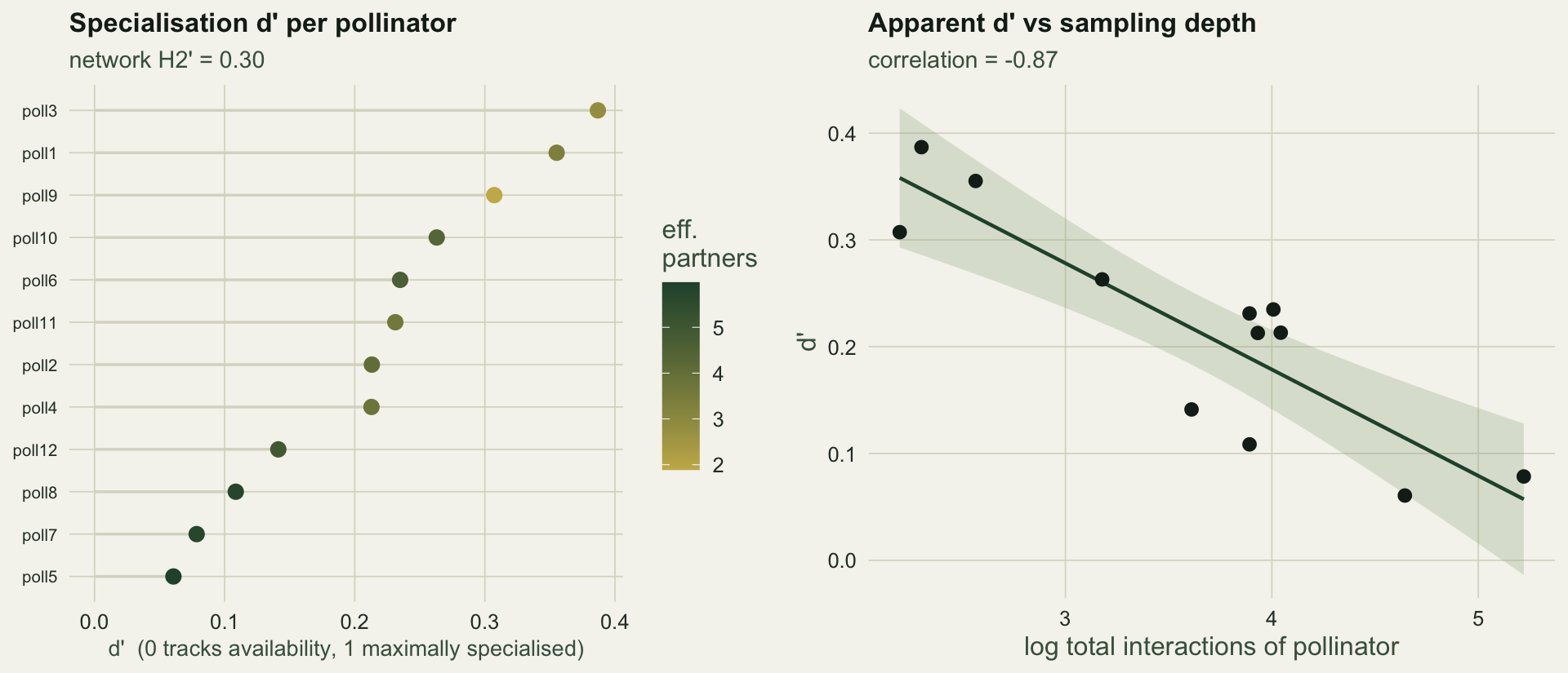
Across pollinators d' runs from `r sprintf("%.2f", min(dprime_poll))` to `r sprintf("%.2f", max(dprime_poll))`, averaging `r sprintf("%.2f", mean(dprime_poll))`. A value near zero means the species visits plants roughly in proportion to how common those plants are; a value of one would mean it monopolises its plants: it visits only them, and no other pollinator visits them at all.
```{r}
#| label: fig-web
#| echo: false
#| fig-width: 10
#| fig-height: 4.3
#| fig-cap: "Left: the interaction matrix, shaded by number of visits. Right: the effective number of plant partners for each pollinator, ranked; the network generality is their interaction-weighted mean."
#| fig-alt: "A twelve by ten heatmap of visit counts, and a ranked lollipop plot of effective plant partners per pollinator rising from about two to about six."
dfm <- data.frame(
poll = factor(rep(rownames(W), times = P), levels = rev(rownames(W))),
plant = factor(rep(colnames(W), each = A), levels = colnames(W)),
n = as.vector(W))
pa <- ggplot(dfm, aes(plant, poll, fill = n)) +
geom_tile(colour = te_paper, linewidth = 0.4) +
scale_fill_gradient(low = te_paper, high = te_forest, name = "visits") +
labs(title = "Interaction matrix", x = "plant species", y = "pollinator species") +
theme_te() + theme(axis.text.x = element_text(angle = 45, hjust = 1, size = rel(0.8)),
axis.text.y = element_text(size = rel(0.8)))
dfg <- data.frame(poll = names(eff_plants), eff = eff_plants)
dfg <- dfg[order(dfg$eff), ]; dfg$poll <- factor(dfg$poll, levels = dfg$poll)
pb <- ggplot(dfg, aes(eff, poll)) +
geom_segment(aes(x = 0, xend = eff, y = poll, yend = poll), colour = te_line, linewidth = 0.6) +
geom_point(colour = te_forest, size = 2.6) +
labs(title = "Generality per pollinator", x = "effective no. of plant partners", y = NULL,
subtitle = sprintf("network generality = %.2f", generality)) +
theme_te() + theme(axis.text.y = element_text(size = rel(0.8)))
grid.newpage(); pushViewport(viewport(layout = grid.layout(1, 2)))
print(pa, vp = viewport(layout.pos.row = 1, layout.pos.col = 1))
print(pb, vp = viewport(layout.pos.row = 1, layout.pos.col = 2))
```
## The honest limit: sampling depth leaks into specialisation
The reason H2' and d' are preferred over connectance is that they standardise against the marginal totals, which soaks up part of the abundance and effort signal. Part, not all. A species seen only a few times cannot look like a generalist: with two or three interactions its d' is pulled upward whether or not it is genuinely choosy. The chunk below measures how much of that is left in this web.
```{r}
#| label: sampling-confound
conf     <- cor(log(rs), dprime_poll)
conf_raw <- cor(log(rs), apply(W, 1, d_raw))   # the divergence before rescaling
round(c(dprime = conf, raw_divergence = conf_raw), 3)
```
The correlation between a pollinator's log total interactions and its d' is `r sprintf("%.2f", conf)`: the thinly seen pollinators tend to score a little higher, but the trend is weak and, with only `r A` pollinators, uncertain. The raw divergence, before each species' ceiling rescales it, tracks sampling far more closely (`r sprintf("%.2f", conf_raw)`), so the rescaling absorbs much of the sampling signal, though not all of it. Some of what remains is real, because the pollinators whose niche position sits near the ends of the plant axis reach fewer plants and are also seen less often in this model, but from the matrix alone the genuine specialists and the under-sampled species cannot be told apart, and both inflate d'. This is the recurring caution in network analysis (Bluthgen 2010; Frund et al 2016), and it sets up the next two posts.
```{r}
#| label: fig-dprime
#| echo: false
#| fig-width: 10
#| fig-height: 4.3
#| fig-cap: "Left: d' for each pollinator, ranked and coloured by effective partners. Right: apparent d' against how many interactions the pollinator was seen making; poorly sampled species score slightly higher on average, with wide scatter."
#| fig-alt: "A ranked lollipop plot of d' per pollinator, and a scatter of d' against log total interactions showing a weak downward trend with wide scatter."
dfd <- data.frame(poll = names(dprime_poll), dprime = dprime_poll,
eff = eff_plants[names(dprime_poll)])
dfd <- dfd[order(dfd$dprime), ]; dfd$poll <- factor(dfd$poll, levels = dfd$poll)
pc <- ggplot(dfd, aes(dprime, poll, colour = eff)) +
geom_segment(aes(x = 0, xend = dprime, y = poll, yend = poll), colour = te_line, linewidth = 0.6) +
geom_point(size = 2.8) +
scale_colour_gradient(low = te_gold, high = te_forest, name = "eff.\npartners") +
labs(title = "Specialisation d' per pollinator", y = NULL,
x = "d' (0 tracks availability, 1 maximally specialised)",
subtitle = sprintf("network H2' = %.2f", H2prime)) +
theme_te() + theme(axis.text.y = element_text(size = rel(0.8)),
axis.title.x = element_text(size = rel(0.85)))
dfs <- data.frame(logtot = log(rs), dprime = dprime_poll)
pd <- ggplot(dfs, aes(logtot, dprime)) +
geom_smooth(method = "lm", formula = y ~ x, se = TRUE, colour = te_forest, fill = te_sage,
alpha = 0.25, linewidth = 0.8) +
geom_point(colour = te_ink, size = 2.4) +
labs(title = "Apparent d' vs sampling depth", x = "log total interactions of pollinator",
y = "d'", subtitle = sprintf("correlation = %.2f", conf)) +
theme_te()
grid.newpage(); pushViewport(viewport(layout = grid.layout(1, 2)))
print(pc, vp = viewport(layout.pos.row = 1, layout.pos.col = 1))
print(pd, vp = viewport(layout.pos.row = 1, layout.pos.col = 2))
```
## Where this leaves you
Connectance and link counts describe a web but cannot be compared across webs of different size or effort. The quantitative descriptors, generality and vulnerability, count effective partners and shrug off stray links. H2' and d' standardise against the marginal totals and travel better, but they are still not immune to sampling: a thinly seen species drifts toward apparent specialisation. Two questions follow. Is an observed value larger than a random web with the same totals would give, which is the job of a null model? And how much does the number move as sampling changes? Those are the subjects of the next posts on [null models for interaction networks](../null-models-for-interaction-networks/) and [checking a network analysis](../checking-a-network-analysis/).
## References
Bersier L-F, Banasek-Richter C, Cattin M-F 2002 Ecology 83(9):2394-2407 (10.1890/0012-9658(2002)083[2394:QDOFWM]2.0.CO;2)
Bluthgen N, Menzel F, Bluthgen N 2006 BMC Ecology 6:9 (10.1186/1472-6785-6-9)
Bluthgen N 2010 Basic and Applied Ecology 11(3):185-195 (10.1016/j.baae.2010.01.001)
Dormann CF, Frund J, Bluthgen N, Gruber B 2009 The Open Ecology Journal 2:7-24 (10.2174/1874213000902010007)
Frund J, McCann KS, Williams NM 2016 Oikos 125(4):502-513 (10.1111/oik.02256)
## Related tutorials
- [Food web structure: connectance and trophic level](../food-web-structure-connectance/)
- [Co-occurrence null models](../co-occurrence-null-models/)
- [Modularity in ecological networks](../modularity-in-ecological-networks/)
- [Null models for interaction networks](../null-models-for-interaction-networks/)