Modularity in ecological networks

Barber’s bipartite modularity, a hand-coded label-propagation module finder, the c-z role plot and a null-model test of significance, all in base R on a plant-pollinator web.

Many interaction webs are not a uniform mesh: species cluster into compartments that interact heavily within and sparsely between, a pattern read as a signature of shared traits, phylogeny or coevolutionary history. Modularity puts a number on that clustering, and the module a species sits in, together with how it bridges to other modules, gives each species a role. This post codes the bipartite modularity of Barber (2007), a label-propagation finder in the spirit of Beckett (2016), and the c-z role plot of Guimera and Amaral (2005) as used for pollination networks by Olesen et al (2007), then tests whether the modularity is more than a random web would show. Everything runs in base R.

A web with built-in compartments

The test web has three latent compartments: pollinators and plants each fall into one of three groups, interactions within a group are strong, and a small share leak across groups. Poisson counts turn the expected rates into an observed matrix.

set.seed(4261)
A0 <- 18L; P0 <- 15L; K <- 3L
poll_grp  <- sort(sample(rep(seq_len(K), length.out = A0)))
plant_grp <- sort(sample(rep(seq_len(K), length.out = P0)))
poll_ab   <- exp(rnorm(A0, 0, 0.4)); plant_ab <- exp(rnorm(P0, 0, 0.4))
lam <- outer(poll_ab, plant_ab) * ifelse(outer(poll_grp, plant_grp, "==") == 1, 1.0, 0.11)
lam <- lam / sum(lam) * 660
W <- matrix(rpois(A0 * P0, lam), A0, P0)
rownames(W) <- paste0("A", seq_len(A0)); colnames(W) <- paste0("P", seq_len(P0))
W <- W[rowSums(W) > 0, colSums(W) > 0, drop = FALSE]
A <- nrow(W); P <- ncol(W); m <- sum(W)
c(pollinators = A, plants = P, interactions = m, connectance = round(sum(W > 0) / (A * P), 3))

 pollinators       plants interactions  connectance 
      18.000       15.000      663.000        0.663 

The web has 18 pollinators, 15 plants and 663 interactions, with connectance 0.66.

Barber’s bipartite modularity

Modularity compares the weight inside modules against what the row and column totals alone would put there. For a bipartite web the modularity matrix is B, with one entry per cell: the observed weight minus the weight expected if interactions were spread in proportion to the marginal totals. Given a labelling that assigns every pollinator and plant to a module, the modularity Q is the sum of B over all pollinator-plant pairs that share a module, divided by the grand total.

ki <- rowSums(W); dj <- colSums(W)
Bmat <- W - outer(ki, dj) / m
Qbip <- function(rl, cl) {
  q <- 0
  for (i in seq_len(A)) { same <- which(cl == rl[i]); if (length(same)) q <- q + sum(Bmat[i, same]) }
  q / m
}

A random labelling scores near zero; a good labelling collects the positive entries of B into blocks and pushes Q up. Finding that labelling is the search problem.

Finding modules by label propagation

The finder alternates two update rules until the labels settle. Each pollinator adopts the module label of the columns it fits best, meaning the label maximising the sum of its B entries over that module’s plants; each plant then does the same over pollinators. Because the landscape has local optima, the search restarts from many random labellings and keeps the best.

lpawb <- function(seed) {
  set.seed(seed)
  nl <- A + P
  rl <- sample(seq_len(nl), A, replace = TRUE)
  cl <- sample(seq_len(nl), P, replace = TRUE)
  repeat {
    changed <- FALSE
    for (i in seq_len(A)) {
      labs <- unique(cl); score <- sapply(labs, function(cc) sum(Bmat[i, cl == cc]))
      best <- labs[which.max(score)]; if (best != rl[i]) { rl[i] <- best; changed <- TRUE }
    }
    for (j in seq_len(P)) {
      labs <- unique(rl); score <- sapply(labs, function(cc) sum(Bmat[rl == cc, j]))
      best <- labs[which.max(score)]; if (best != cl[j]) { cl[j] <- best; changed <- TRUE }
    }
    if (!changed) break
  }
  list(rl = rl, cl = cl, Q = Qbip(rl, cl))
}
runs <- lapply(seq_len(40L), function(s) lpawb(1000 + s))
Qs   <- vapply(runs, `[[`, numeric(1), "Q")
best <- runs[[which.max(Qs)]]
alllab <- unique(c(best$rl, best$cl)); map <- setNames(seq_along(alllab), alllab)
rlab <- map[as.character(best$rl)]; clab <- map[as.character(best$cl)]
Qobs <- best$Q; nmod <- length(unique(c(rlab, clab)))
c(Q = round(Qobs, 3), modules = nmod, restart_low = round(min(Qs), 3), restart_high = round(max(Qs), 3))

           Q      modules  restart_low restart_high 
       0.468        3.000        0.420        0.468 

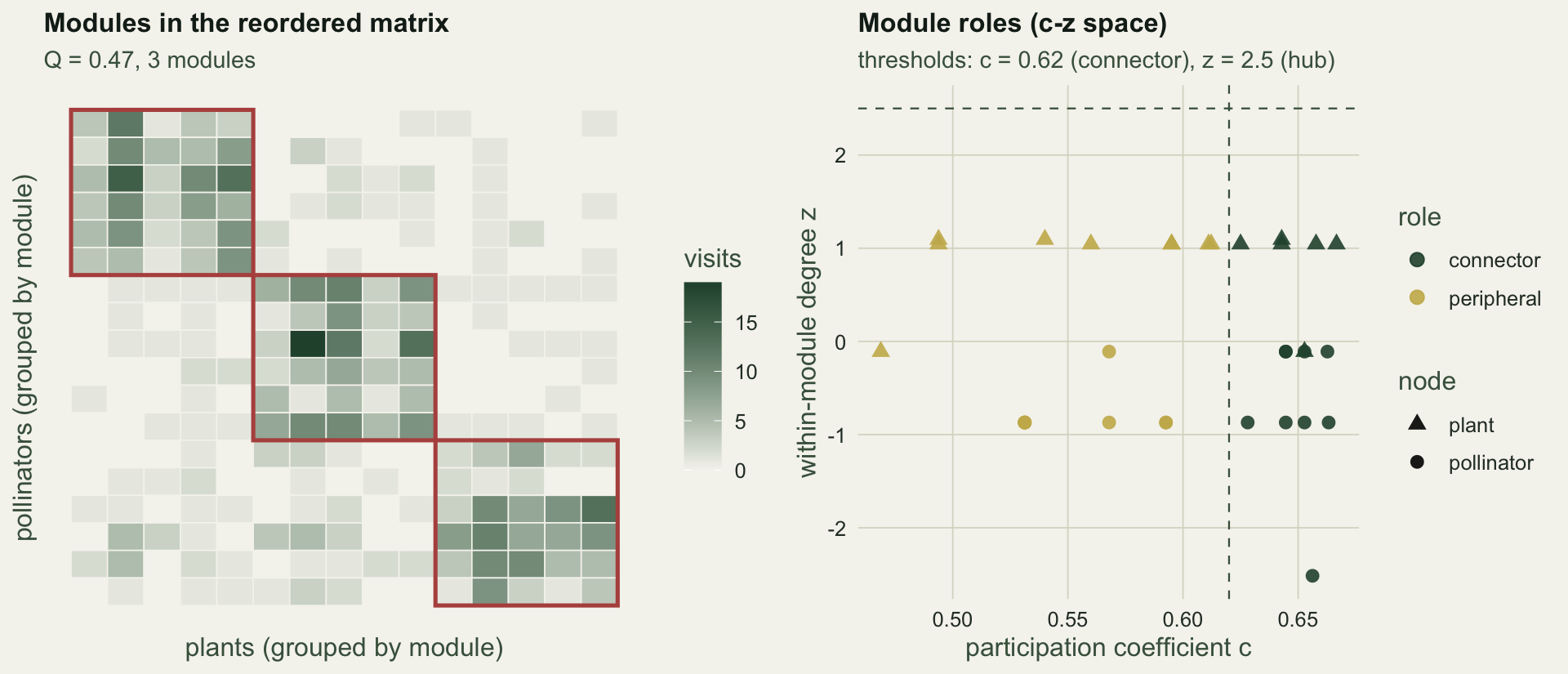
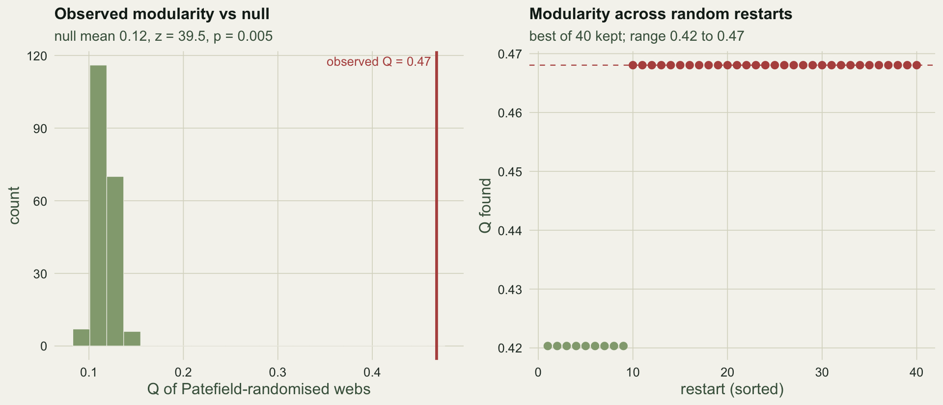
The best of 40 restarts reaches Q = 0.47 with 3 modules, and recovers the three planted compartments cleanly. The restarts do not all agree: they range from 0.42 to 0.47, which is the first caveat. Module detection is a heuristic search, so a single run can return a worse partition, and the reported modularity is the maximum over many attempts rather than a guaranteed optimum.

Species roles: connectors, hubs and peripherals

With modules in hand, two numbers describe how a species sits in the web. The within-module degree z is how many links a species has to its own module, standardised against the other members of that module: a species with far more within-module links than its peers has a high z and anchors the module. The participation coefficient c measures how evenly a species spreads its links across modules: zero if all its links stay in one module, approaching one if they are shared out. Following Olesen et al (2007), a species with c above 0.62 is a connector, one with z above 2.5 is a module hub, both make it a network hub, and neither leaves it peripheral.

Adj <- (W > 0) * 1L
node_mod <- c(rlab, clab); N <- A + P
G <- matrix(0L, N, N); G[1:A, (A + 1):N] <- Adj; G[(A + 1):N, 1:A] <- t(Adj)
deg <- rowSums(G)
zc_mat <- t(vapply(seq_len(N), function(v) {
  s <- node_mod[v]; kis <- sum(G[v, node_mod == s]); members <- which(node_mod == s)
  kv <- vapply(members, function(u) sum(G[u, node_mod == s]), numeric(1))
  z  <- if (sd(kv) > 0) (kis - mean(kv)) / sd(kv) else 0
  ct <- vapply(sort(unique(node_mod)), function(t) sum(G[v, node_mod == t]), numeric(1))
  cpar <- if (deg[v] > 0) 1 - sum((ct / deg[v])^2) else 0
  c(z = z, c = cpar)
}, numeric(2)))
role <- ifelse(zc_mat[, "z"] > 2.5 & zc_mat[, "c"] > 0.62, "network hub",
        ifelse(zc_mat[, "z"] > 2.5, "module hub",
        ifelse(zc_mat[, "c"] > 0.62, "connector", "peripheral")))
role_tab <- list(zc = zc_mat, role = role)
n_conn <- sum(role == "connector"); n_periph <- sum(role == "peripheral")
n_hub  <- sum(grepl("hub", role))
c(connector = n_conn, peripheral = n_periph, hub = n_hub)

 connector peripheral        hub 
        15         18          0 

Here 15 species are connectors, 18 are peripheral and 0 are hubs. The absence of hubs is common in real pollination webs: modules are held together more by species that bridge across them than by dominant within-module anchors.

Figure 1: Left: the interaction matrix with rows and columns reordered by module, blocks outlined. Right: each species placed by its participation coefficient c and within-module degree z, with the connector and hub thresholds of Olesen et al (2007).

Is the web more modular than chance?

A raw Q cannot be read on its own, because a random web with the same row and column totals also has positive modularity. The honest comparison is against a null. The Patefield algorithm, available in base R as r2dtable, draws random matrices holding the marginal totals fixed; running the same module finder on each gives a null distribution for Q.

set.seed(99)
nnull <- 199L
nulls <- r2dtable(nnull, ki, dj)
Qnull <- vapply(seq_len(nnull), function(b) {
  Wn <- nulls[[b]]; kn <- rowSums(Wn); dn <- colSums(Wn); Bn <- Wn - outer(kn, dn) / sum(Wn)
  Aq <- nrow(Wn); Pq <- ncol(Wn)
  QN <- function(rl, cl) { q <- 0; for (i in seq_len(Aq)) { s <- which(cl == rl[i]); if (length(s)) q <- q + sum(Bn[i, s]) }; q / sum(Wn) }
  lp <- function(seed) {
    set.seed(seed); nl <- Aq + Pq; rl <- sample(nl, Aq, TRUE); cl <- sample(nl, Pq, TRUE)
    repeat { ch <- FALSE
      for (i in seq_len(Aq)) { L <- unique(cl); sc <- sapply(L, function(cc) sum(Bn[i, cl == cc])); bb <- L[which.max(sc)]; if (bb != rl[i]) { rl[i] <- bb; ch <- TRUE } }
      for (j in seq_len(Pq)) { L <- unique(rl); sc <- sapply(L, function(cc) sum(Bn[rl == cc, j])); bb <- L[which.max(sc)]; if (bb != cl[j]) { cl[j] <- bb; ch <- TRUE } }
      if (!ch) break }
    QN(rl, cl)
  }
  max(vapply(1:6, function(s) lp(500 * b + s), numeric(1)))
}, numeric(1))
z_mod <- (Qobs - mean(Qnull)) / sd(Qnull)
p_mod <- (1 + sum(Qnull >= Qobs)) / (nnull + 1)
c(null_mean = round(mean(Qnull), 3), null_sd = round(sd(Qnull), 3),
  observed = round(Qobs, 3), z = round(z_mod, 2), p = round(p_mod, 3))

null_mean   null_sd  observed         z         p 
    0.117     0.009     0.468    39.530     0.005 

The randomised webs cluster around Q = 0.12, well below the observed 0.47, giving a z-score of 39.5 and p = 0.005. The web is modular beyond what its totals force. Without the null the raw 0.47 would be uninterpretable, since even structureless webs return a positive value.

Figure 2: Left: observed modularity against the distribution of Q from Patefield-randomised webs with the same totals. Right: the modularity found on each of the random restarts, sorted, showing that the search does not always reach the best value.

Where this leaves you

A web can be split into modules, the split scored with Barber’s Q, and each species given a role from its within-module degree and its cross-module participation. Three cautions travel with those numbers. The search is heuristic, so the modularity is a best-of-many rather than a proven optimum. The raw Q means nothing without a null, because random webs are modular too. And, as the next posts show, Q and the role thresholds shift with the size and sampling of the web, so values are best compared as departures from a null rather than head to head. Those threads continue in null models for interaction networks and checking a network analysis.

References

Barber, M. J. (2007). Modularity and community detection in bipartite networks. Physical Review E, 76(6), 066102. https://doi.org/10.1103/PhysRevE.76.066102

Beckett, S. J. (2016). Improved community detection in weighted bipartite networks. Royal Society Open Science, 3(1), 140536. https://doi.org/10.1098/rsos.140536

Dormann, C. F. and Strauss, R. (2014). A method for detecting modules in quantitative bipartite networks. Methods in Ecology and Evolution, 5(1), 90-98. https://doi.org/10.1111/2041-210X.12139

Guimera, R. and Amaral, L. A. N. (2005). Functional cartography of complex metabolic networks. Nature, 433(7028), 895-900. https://doi.org/10.1038/nature03288

Newman, M. E. J. and Girvan, M. (2004). Finding and evaluating community structure in networks. Physical Review E, 69(2), 026113. https://doi.org/10.1103/PhysRevE.69.026113

Olesen, J. M., Bascompte, J., Dupont, Y. L. and Jordano, P. (2007). The modularity of pollination networks. Proceedings of the National Academy of Sciences, 104(50), 19891-19896. https://doi.org/10.1073/pnas.0706375104

Related tutorials

• Bipartite network metrics from scratch
• Nestedness and the NODF metric
• Null models for interaction networks
• Checking a network analysis

## References

Barber MJ 2007 Physical Review E 76(6):066102 (10.1103/PhysRevE.76.066102)
Beckett SJ 2016 Royal Society Open Science 3(1):140536 (10.1098/rsos.140536)
Dormann CF and Strauss R 2014 Methods in Ecology and Evolution 5(1):90-98 (10.1111/2041-210X.12139)
Guimera R and Amaral LAN 2005 Nature 433(7028):895-900 (10.1038/nature03288)
Newman MEJ and Girvan M 2004 Physical Review E 69(2):026113 (10.1103/PhysRevE.69.026113)