library(ggplot2)

te_pal <- list(forest = "#275139", green = "#2f8f63", sage = "#93a87f",
               clay = "#b5534e", gold = "#cda23f", line = "#dad9ca",
               ink = "#16241d", paper = "#f5f4ee")

theme_te <- function() {
  theme_minimal(base_size = 12) +
    theme(panel.grid.minor = element_blank(),
          panel.grid.major = element_line(colour = "#e7e6dc"),
          plot.background = element_rect(fill = "#f5f4ee", colour = NA),
          panel.background = element_rect(fill = "#f5f4ee", colour = NA),
          plot.title = element_text(face = "bold", colour = te_pal$ink),
          axis.title = element_text(colour = "#2c3a31"),
          axis.text = element_text(colour = "#2c3a31"))
}Residuals as a variable: the two-step trap
R
regression
collinearity
model diagnostics
ecology tutorial
Residualising one predictor on another to dodge collinearity in R: what the two-step estimator really measures, and why its interval fails a coverage check.
A jackdaw colony of 200 colour-ringed adults, watched at a supplementary feeding station over four breeding seasons. Observers ran ninety-six recording sessions and wrote down which ringed birds were present at each one, so every bird carries a sighting count. From the co-occurrence pattern the fieldworkers built an association network and scored each bird’s social strength. Every bird was also weighed and its tarsus measured at ringing, and every bird’s nest was followed to fledging.
Two questions come out of that dataset, and the same statistical move gets made for both. Does a bird’s social position predict how many young it fledges? And does body condition differ between the two woodland patches the colony feeds in? For the first question, social strength and sighting count are correlated at about 0.85, because a bird that turns up at more sessions has more chances to be scored as associating with somebody. For the second, mass depends on skeletal size and the two patches hold birds of appreciably different size. In both cases the analyst regresses the awkward variable on the nuisance variable, keeps the residual, and carries that residual into the next model as if it were a measured quantity.
This is one of the most widespread manoeuvres in ecology. Body condition as the residual of mass on a length measurement. A centrality metric residualised on sighting effort. A diversity index residualised on sampling intensity. Range size residualised on body mass. The stated reason is almost always the same: the two variables are correlated, putting both in one model is said to be unsafe, so one of them is cleaned of the other first. The move feels conservative. It looks like taking the confound seriously.
What follows measures it, on synthetic data with the generating model known, so every error is a distance from a number that was set. The post asks four things of the two-step: what its slope actually estimates, whether its interval covers at the nominal rate, what the collinearity it was meant to fix would have cost in one model, and what the honest version costs when the residual really is the quantity of interest.
Three posts on this blog sit next to this one and none of them prices the move. Collinearity and VIF in ecological regression is the diagnostic side: it computes the variance inflation factor by hand and says what a large one means, but it stops before the question of what analysts then do about it. Offsets for rates and densities in Poisson GLMs is the correct way to carry sampling effort into a count model, by putting log effort in as a fixed-coefficient term rather than residualising it out beforehand. And network centrality and sampling effort is a live tutorial here that names the residual route as one of two honest ways forward, and attaches no price to it at all. This post supplies the price, and the two should be read together.
Four routes to one coefficient
The generating model is the plainest thing that can carry the problem. Sighting effort is standardised to mean zero and unit variance; social strength is built to correlate with it at a set value; the fledging count depends on both, the strength effect being the quantity of interest and the effort effect a real influence on breeding output rather than a pure artefact. Nothing is non-linear, nothing is measured with error, the errors are Gaussian. Every failure below happens in the friendliest possible world.
n_bird <- 200
rho_main <- 0.85
b_str <- 0.40
b_eff <- 0.55
sd_fled <- 1

gen_col <- function(rho, b1v) {
  eff <- rnorm(n_bird)
  strg <- rho * eff + sqrt(1 - rho^2) * rnorm(n_bird)
  data.frame(eff = eff, strg = strg,
             fled = 3 + b1v * strg + b_eff * eff + rnorm(n_bird, 0, sd_fled))
}

print(c(birds = n_bird, correlation = rho_main,
        strength_effect = b_str, effort_effect = b_eff,
        residual_sd = sd_fled))
birds correlation strength_effect effort_effect residual_sd
200.00 0.85 0.40 0.55 1.00 There are 200 birds, the correlation between social strength and sighting effort is 0.85, the true partial effect of strength on fledglings is 0.4 and the true partial effect of effort is 0.55. Four ways of getting at the strength coefficient are in circulation, and it is worth writing all four down before running any of them.
The first is the one model: regress fledglings on strength and effort together and read the strength coefficient. The second is the move this post is about: regress strength on effort, keep the residual, then regress fledglings on that residual alone. The third is the mirror image, the one that produces a body condition index: keep the residual of fledglings on effort and regress it on raw strength. The fourth residualises both sides.
set.seed(20260804)
d1 <- gen_col(rho_main, b_str)

m_full <- lm(fled ~ strg + eff, data = d1)
res_strg <- residuals(lm(strg ~ eff, data = d1))
res_fled <- residuals(lm(fled ~ eff, data = d1))

m_pred <- lm(d1$fled ~ res_strg)
m_resp <- lm(res_fled ~ d1$strg)
m_fwl <- lm(res_fled ~ res_strg)
m_marg <- lm(fled ~ strg, data = d1)

b_one <- unname(coef(m_full)[2])
b_pred <- unname(coef(m_pred)[2])
b_resp <- unname(coef(m_resp)[2])
b_fwl <- unname(coef(m_fwl)[2])
b_marg <- unname(coef(m_marg)[2])
r2_stage1 <- summary(lm(strg ~ eff, data = d1))$r.squared

print(round(c(one_model = b_one, predictor_residualised = b_pred,
              response_residualised = b_resp, both_residualised = b_fwl,
              marginal = b_marg), 8))
one_model predictor_residualised response_residualised
0.5752909 0.5752909 0.1501157
both_residualised marginal
0.5752909 1.0367607 print(c(diff_predictor = formatC(abs(b_pred - b_one), format = "e", digits = 3),
diff_both = formatC(abs(b_fwl - b_one), format = "e", digits = 3)))diff_predictor diff_both
"3.331e-16" "5.551e-16" print(round(c(stage1_r_squared = r2_stage1, one_minus_r2 = 1 - r2_stage1,
one_model_times_one_minus_r2 = b_one * (1 - r2_stage1),
response_route = b_resp), 8)) stage1_r_squared one_minus_r2
0.7390612 0.2609388
one_model_times_one_minus_r2 response_route
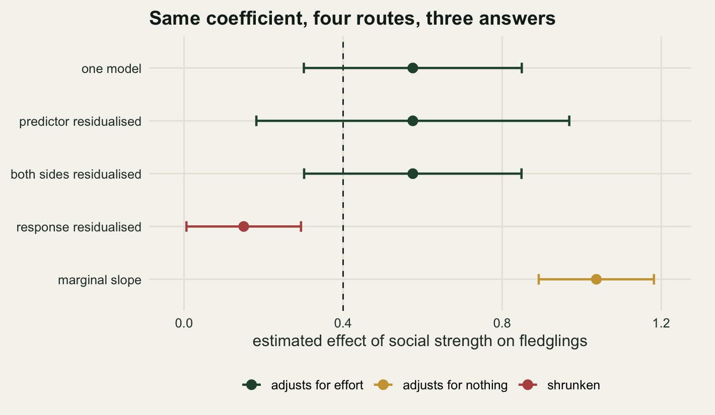
0.1501157 0.1501157 Three of the four numbers are the same number. The one model gives 0.575291, residualising the predictor gives the same to 3.33e-16, and residualising both sides gives the same to 5.55e-16. Those are floating-point differences, not statistical ones. The fourth number, from residualising the response, is 0.150116, and it is not close.
That pattern is not luck and it is not a property of this dataset. It is the Frisch-Waugh-Lovell theorem, first written down by Frisch and Waugh (1933) for the problem of detrending time series and given its modern short proof by Lovell (2008). Write \(M_2\) for the operator that regresses anything on an intercept and effort and returns the residual, and let \(\tilde{x}_1 = M_2 x_1\) and \(\tilde{y} = M_2 y\) be the residualised strength and the residualised fledging count. The theorem says
\[\hat\beta_1 \;=\; \frac{\tilde{x}_1^{\top} \tilde{y}}{\tilde{x}_1^{\top} \tilde{x}_1}\]
where \(\hat\beta_1\) is the coefficient on strength from the two-predictor regression. So residualising both sides recovers the partial slope exactly.
The reason residualising only the predictor also works is one line further. Because \(M_2\) is a projection, \(\tilde{x}_1^{\top} \tilde{y} = \tilde{x}_1^{\top} M_2 y = \tilde{x}_1^{\top} y\): the residual \(\tilde{x}_1\) is already orthogonal to effort, so the part of the fledging count that effort explains cannot enter the numerator whether it is removed first or not. Carrying an unresidualised response into the second stage changes nothing about the point estimate.
The response-only route is a different object. Regressing \(\tilde{y}\) on raw strength divides by the wrong quantity:
\[\hat\beta_1^{\text{resp}} \;=\; \frac{\tilde{x}_1^{\top} y}{x_1^{\top} x_1} \;=\; \left(1 - R^2_{1|2}\right) \hat\beta_1\]
with strength centred, and \(R^2_{1|2}\) the fit of strength on effort. The denominator is the total variance of strength where it should have been the variance of strength that effort does not explain. The result is the partial slope shrunk towards zero by exactly the fraction of the predictor’s variance that the nuisance variable accounts for. In this dataset that fraction is 0.7391, so the response route returns 0.575291 times 0.2609, which is 0.150116, and the fitted value is 0.150116.
One clarification about the direction of the shrinkage, because the folk version of this warning gets it backwards. The residual route is often described as leaving the estimate somewhere between the partial slope and the marginal one. It does not. The marginal slope here is 1.0368, well above the partial slope, and the response route lands below both. Whatever the two-step is doing, it is not a partial correction of the unadjusted relationship.
Two thousand colonies
One dataset settles the algebra and nothing else. The replicate study redraws the whole colony two thousand times, fits all four routes each time, and records the estimate and the standard error the software prints. It runs twice: once with the true strength effect set to 0.4, to measure bias, interval coverage and power, and once with it set to zero, to measure the rate at which each route claims an effect that is not there.
three_routes <- function(dd) {
  sf <- summary(lm(fled ~ strg + eff, data = dd))$coefficients
  rs <- residuals(lm(strg ~ eff, data = dd))
  rf <- residuals(lm(fled ~ eff, data = dd))
  sp <- summary(lm(dd$fled ~ rs))$coefficients
  sr <- summary(lm(rf ~ dd$strg))$coefficients
  sw <- summary(lm(rf ~ rs))$coefficients
  c(sf[2, 1], sf[2, 2], sp[2, 1], sp[2, 2],
    sr[2, 1], sr[2, 2], sw[2, 1], sw[2, 2])
}

n_rep <- 2000
set.seed(80401)
alt <- t(replicate(n_rep, three_routes(gen_col(rho_main, b_str))))
set.seed(80402)
nul <- t(replicate(n_rep, three_routes(gen_col(rho_main, 0))))

t_full <- qt(0.975, n_bird - 3)
t_two <- qt(0.975, n_bird - 2)
tv <- c(t_full, t_two, t_two, t_two)
idx_e <- c(1, 3, 5, 7)
idx_s <- c(2, 4, 6, 8)

rep_tab <- data.frame(
  route = c("one model", "predictor residualised",
            "response residualised", "both sides residualised"),
  est = colMeans(alt[, idx_e]),
  spread = apply(alt[, idx_e], 2, sd),
  mean_se = colMeans(alt[, idx_s]),
  coverage = vapply(seq_along(idx_e), function(j)
    mean(abs(alt[, idx_e[j]] - b_str) < tv[j] * alt[, idx_s[j]]), numeric(1)),
  power = vapply(seq_along(idx_e), function(j)
    mean(abs(alt[, idx_e[j]] / alt[, idx_s[j]]) > tv[j]), numeric(1)),
  type_i = vapply(seq_along(idx_e), function(j)
    mean(abs(nul[, idx_e[j]] / nul[, idx_s[j]]) > tv[j]), numeric(1)))

print(round(rep_tab[, -1], 5))
est spread mean_se coverage power type_i
1 0.40132 0.13155 0.13530 0.9520 0.8485 0.0455
2 0.40132 0.13155 0.18139 0.9915 0.6290 0.0230
3 0.11141 0.03877 0.07212 0.0020 0.1995 0.0005
4 0.40132 0.13155 0.13496 0.9510 0.8485 0.0455print(rep_tab$route)[1] "one model" "predictor residualised"
[3] "response residualised" "both sides residualised"print(c(max_gap_predictor =
formatC(max(abs(alt[, 1] - alt[, 3])), format = "e", digits = 3),
max_gap_both =
formatC(max(abs(alt[, 1] - alt[, 7])), format = "e", digits = 3)))max_gap_predictor max_gap_both
"2.609e-15" "2.470e-15" print(round(c(shrink_factor = 1 - rho_main^2,
predicted_response_route = mean(alt[, 1]) * (1 - rho_main^2),
measured_response_route = mean(alt[, 5])), 5)) shrink_factor predicted_response_route measured_response_route
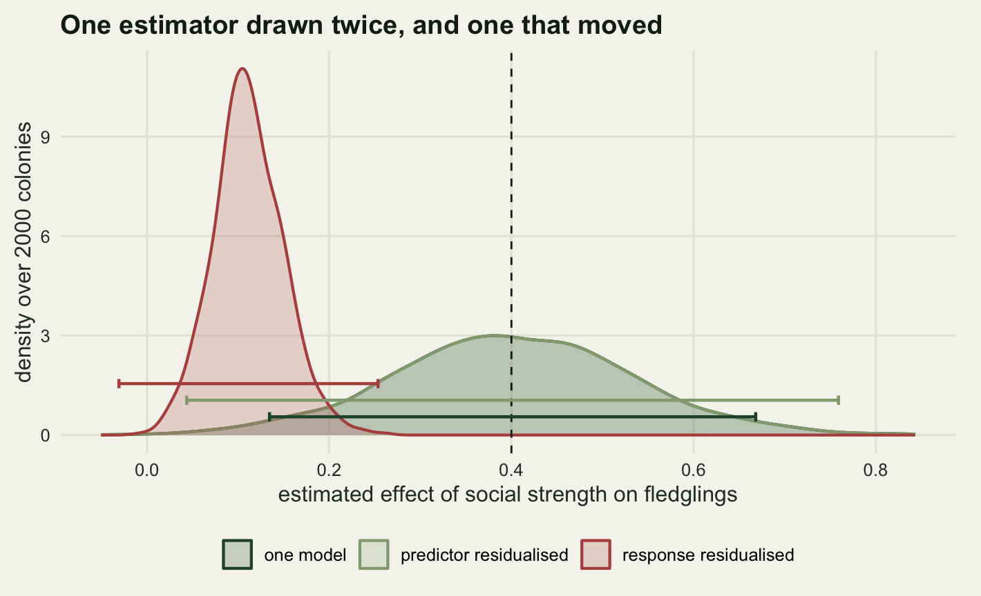
0.27750 0.11137 0.11141 Over 2000 colonies the one model averages 0.4013 against a truth of 0.4. Residualising the predictor averages exactly the same value: the largest gap between the two estimates over all 2000 replicates is 2.61e-15. Residualising both sides agrees to 2.47e-15. There is no simulation error in those two statements, because there is nothing being estimated twice: the three routes are the same arithmetic written three ways.
The response route averages 0.1114. The shrinkage factor \(1 - \rho^2\) is 0.2775 at this correlation, so the predicted value is 0.11137 and the measured one is 0.11141. The bias is -0.2886, which is 72.15 per cent of the effect being chased, removed by nothing more than the choice of which side to residualise.
Now the intervals, where the predictor route parts company with the two others that share its point estimate.
print(round(c(predictor_se_ratio = rep_tab$mean_se[2] / rep_tab$mean_se[1],
              response_se_ratio = rep_tab$mean_se[3] / rep_tab$mean_se[1],
              power_lost_predictor = rep_tab$power[1] - rep_tab$power[2],
              power_lost_response = rep_tab$power[1] - rep_tab$power[3]), 5))
predictor_se_ratio response_se_ratio power_lost_predictor
1.34065 0.53301 0.21950
power_lost_response
0.64900 The one model reports a mean standard error of 0.1353 against an actual spread of estimates across colonies of 0.1315. Those two agree, which is what an honest standard error looks like, and coverage comes out at 95.2 per cent against a nominal 95.
The predictor route has the same spread, 0.1315, because it is the same estimator, but reports a standard error of 0.1814, a factor of 1.341 too large. Its second stage leaves effort out of the model, so everything effort does to the fledging count lands in the residual variance and inflates the standard error. Coverage is 99.15 per cent, which sounds harmless until the power column is read: 62.9 per cent against the one model’s 84.85 per cent. The move that was supposed to protect the analysis from collinearity throws away 21.95 percentage points of power on a real effect while returning an estimate that differs from the one model’s only in floating point.
The response route reports 0.0721, which is 46.7 per cent narrower than the one model’s interval. That is the reason the move survives: the output looks more precise. Coverage of the true value is 0.2 per cent, on an interval that is short, tight and centred on a number nobody wanted.
One number in that table did not come out as I expected, and it is worth stating plainly because it cuts against the usual warning. The false-positive rate of the response route is 0.05 per cent against a nominal 5, and the predictor route is at 2.3 per cent. Neither is anti-conservative. When the first stage is fitted to the same birds by ordinary least squares, the second stage inherits an interval that is too wide, not too narrow, and under a true null both residual routes reject less often than they should. The failure of the response route is entirely a failure of location: the shrinkage takes the estimate away from the truth, and the interval is too short to follow it back. Its power against a real effect is 19.95 per cent, less than a quarter of the one model’s.
What the collinearity was actually costing
The diagnostic that gets quoted to justify the two-step is the variance inflation factor, sometimes with a condition number alongside it. The word condition is doing double duty in this post: the condition number of a design matrix is a collinearity diagnostic and has nothing to do with a body condition index. Both appear below and they are unrelated.
The variance inflation factor for a predictor is \(1/(1 - R^2)\) where \(R^2\) comes from regressing that predictor on the others, and it says by what factor the variance of its coefficient is multiplied relative to an orthogonal design. The condition number is the ratio of the largest to the smallest singular value of the scaled design matrix. Both are descriptions of the same geometry, and neither says anything about whether an estimator is biased. The sweep below runs the whole replicate study at five correlations and puts the diagnostics beside the thing they are supposed to warn about.
rho_grid <- c(0.5, 0.7, 0.8, 0.9, 0.95)
n_sweep <- 1000

sweep_one <- function(k) {
  set.seed(90500 + k)
  aa <- t(replicate(n_sweep, three_routes(gen_col(rho_grid[k], b_str))))
  set.seed(99000 + k)
  dk <- gen_col(rho_grid[k], b_str)
  sv <- svd(cbind(1, scale(dk$strg), scale(dk$eff)))$d
  data.frame(
    rho = rho_grid[k],
    vif = 1 / (1 - rho_grid[k]^2),
    kappa = max(sv) / min(sv),
    one_hw = t_full * mean(aa[, 2]),
    one_cov = mean(abs(aa[, 1] - b_str) < t_full * aa[, 2]),
    one_pow = mean(abs(aa[, 1] / aa[, 2]) > t_full),
    pred_hw = t_two * mean(aa[, 4]),
    pred_cov = mean(abs(aa[, 3] - b_str) < t_two * aa[, 4]),
    pred_pow = mean(abs(aa[, 3] / aa[, 4]) > t_two),
    resp_est = mean(aa[, 5]),
    resp_hw = t_two * mean(aa[, 6]),
    resp_cov = mean(abs(aa[, 5] - b_str) < t_two * aa[, 6]),
    resp_pow = mean(abs(aa[, 5] / aa[, 6]) > t_two))
}

sweep <- do.call(rbind, lapply(seq_along(rho_grid), sweep_one))
print(round(sweep[, c("rho", "vif", "kappa", "one_hw", "one_cov",
                      "one_pow")], 4))
rho vif kappa one_hw one_cov one_pow
1 0.50 1.3333 1.6250 0.1627 0.952 0.996
2 0.70 1.9608 2.3152 0.1979 0.962 0.979
3 0.80 2.7778 3.1523 0.2343 0.956 0.919
4 0.90 5.2632 4.6169 0.3219 0.944 0.672
5 0.95 10.2564 6.2014 0.4511 0.950 0.428print(round(sweep[, c("rho", "pred_hw", "pred_cov", "pred_pow")], 4)) rho pred_hw pred_cov pred_pow
1 0.50 0.2031 0.980 0.992
2 0.70 0.2565 0.990 0.913
3 0.80 0.3101 0.991 0.780
4 0.90 0.4356 0.986 0.419
5 0.95 0.6152 0.994 0.192print(round(sweep[, c("rho", "resp_est", "resp_hw", "resp_cov",
"resp_pow")], 4)) rho resp_est resp_hw resp_cov resp_pow
1 0.50 0.3013 0.1425 0.737 0.994
2 0.70 0.2043 0.1436 0.182 0.867
3 0.80 0.1463 0.1429 0.014 0.519
4 0.90 0.0760 0.1419 0.000 0.018
5 0.95 0.0405 0.1418 0.000 0.000hw_ratio <- sweep$one_hw / sweep$resp_hw
print(round(c(hw_ratio_lowest_rho = hw_ratio[1],
hw_ratio_highest_rho = hw_ratio[length(hw_ratio)],
resp_hw_range = max(sweep$resp_hw) - min(sweep$resp_hw)), 5)) hw_ratio_lowest_rho hw_ratio_highest_rho resp_hw_range
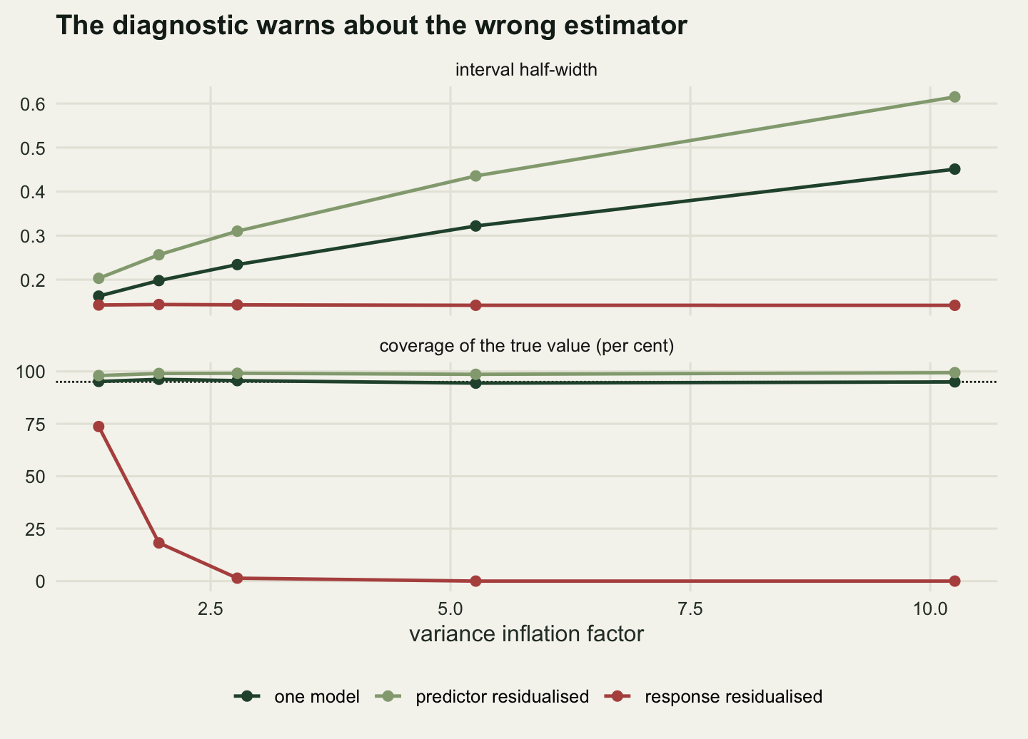
1.14185 3.18179 0.00184 Read the three tables against each other. The variance inflation factor climbs from 1.333 to 10.256 and the condition number from 1.625 to 6.201, so by the inflation factor the design goes from unremarkable to a case that would be flagged in any diagnostic table, while the condition number stays below the values conventionally treated as a warning. What that costs the one model is written in its interval: the half-width goes from 0.1627 to 0.4511, and power against the true effect falls from 99.6 per cent to 42.8 per cent. That is the honest bill for correlated predictors, and coverage stays at 95.2 per cent and 95 per cent at the two ends. The one model is not lying about anything; it is telling the analyst that the data cannot separate the two variables very well.
The response route’s interval half-width barely moves across the whole sweep, from 0.1425 to 0.1418, a total range of 0.00184. At the mildest correlation the one model’s interval is 1.142 times as wide as the two-step’s; at the strongest it is 3.182 times as wide. The worse the collinearity gets, the better the two-step looks, and the reason it looks better is that its denominator is the total variance of strength, which collinearity does not touch. Precision that does not respond to the problem is not precision.
What it buys with that steadiness is written in the coverage column: 73.7 per cent at the mildest correlation, 1.4 per cent in the middle, and 0 per cent at the strongest, where not one interval in a thousand contained the true value. Its estimate shrinks from 0.3013 to 0.0405 against a constant truth of 0.4, and its power against a real effect falls to 0 per cent. The comparison the diagnostics were supposed to inform is variance against bias, and the two-step loses on both terms once coverage is the criterion: it has more bias and, at the correlations where anybody would reach for it, less power as well.
The predictor route sits in between. Its coverage runs from 98 to 99.4 per cent, always above nominal, and its power falls from 99.2 to 19.2 per cent. It gets the right answer and reports it too cautiously, which is defensible and wasteful. This is the arrangement Freckleton (2002) compared with multiple regression for exactly this ecological setting; Garcia-Berthou (2001) made the parallel argument in the analysis of covariance framing the condition-index literature lives in, and Darlington and Smulders (2001) reached it from the behavioural side.
When the first stage is somebody else’s regression
Everything so far had the first stage fitted to the same birds as the second. That is why the two-step’s interval came out too wide rather than too narrow: least squares had already conditioned on the nuisance variable, and the projection that makes the residual is a fixed function of data the second stage is looking at anyway. Change that one detail and the failure changes sign.
Condition indices are often computed from a slope that did not come from the study sample: a published allometric exponent, a museum series, a calibration sample from an earlier year. The fieldworker takes the number, applies it to this year’s birds and analyses the resulting index. This is the generated-regressor problem Pagan (1984) set out, and the second-stage software has no way of knowing one of its inputs was estimated.
The colony’s second question supplies the setting. Body mass and tarsus are both on the log scale, an allometric exponent is estimated from a reference series of 60 birds, the condition index for each study bird is its log mass minus the exponent times its log tarsus, and the question is whether mean condition differs between the two woodland patches. The patches hold birds of appreciably different skeletal size, which is what makes the first-stage slope matter.
m_ref <- 60
n_st <- 200
n_half <- n_st / 2
b_allo <- 3.1
sd_lmass <- 0.055
sd_ltar <- 0.030
mu_ltar <- c(3.780, 3.825)
tau_true <- 0.030
hab <- rep(0:1, each = n_half)

slope1 <- function(xv, yv) {
  xc <- xv - mean(xv)
  sum(xc * (yv - mean(yv))) / sum(xc * xc)
}

sim_cond <- function(tau) {
  ltar_r <- rnorm(m_ref, mean(mu_ltar), sd_ltar)
  lmass_r <- -8.5 + b_allo * ltar_r + rnorm(m_ref, 0, sd_lmass)
  ltar_s <- rnorm(n_st, mu_ltar[hab + 1], sd_ltar)
  lmass_s <- -8.5 + b_allo * ltar_s + tau * hab + rnorm(n_st, 0, sd_lmass)
  list(ltar_r = ltar_r, lmass_r = lmass_r,
       ltar_s = ltar_s, lmass_s = lmass_s)
}

pair_fit <- function(sv) {
  bh <- slope1(sv$ltar_r, sv$lmass_r)
  cidx <- sv$lmass_s - bh * sv$ltar_s
  mm <- summary(lm(cidx ~ hab))$coefficients
  an <- summary(lm(sv$lmass_s ~ sv$ltar_s + hab))$coefficients
  c(mm[2, 1], mm[2, 2], an[3, 1], an[3, 2], bh)
}

print(c(reference_birds = m_ref, study_birds = n_st,
        allometric_exponent = b_allo, true_condition_gap = tau_true))
reference_birds study_birds allometric_exponent true_condition_gap
60.00 200.00 3.10 0.03 print(round(c(log_tarsus_sd_within_patch = sd_ltar,
log_tarsus_gap_between_patches = diff(mu_ltar),
gap_in_within_patch_sds = diff(mu_ltar) / sd_ltar,
log_mass_residual_sd = sd_lmass), 4)) log_tarsus_sd_within_patch log_tarsus_gap_between_patches
0.030 0.045
gap_in_within_patch_sds log_mass_residual_sd
1.500 0.055 The reference series has 60 birds, the study has 200 in two patches of 100, the true allometric exponent is 3.1, and the true difference in condition between the patches is 0.03 on the log scale, or 3.05 per cent in mass. The patches differ in mean log tarsus by 0.045, which is 1.5 within-patch standard deviations: a large difference next to the variation among birds inside a patch, and, as the closed-form term later in this section shows, the quantity that decides how much variance the printed interval leaves out.
n_rep_c <- 1500
set.seed(70301)
cond_alt <- t(replicate(n_rep_c, pair_fit(sim_cond(tau_true))))
set.seed(70302)
cond_nul <- t(replicate(n_rep_c, pair_fit(sim_cond(0))))

t_c2 <- qt(0.975, n_st - 2)
t_c3 <- qt(0.975, n_st - 3)
cond_tab <- data.frame(
  method = c("two-step index", "one model (ANCOVA)"),
  est = c(mean(cond_alt[, 1]), mean(cond_alt[, 3])),
  spread = c(sd(cond_alt[, 1]), sd(cond_alt[, 3])),
  mean_se = c(mean(cond_alt[, 2]), mean(cond_alt[, 4])),
  coverage = c(mean(abs(cond_alt[, 1] - tau_true) < t_c2 * cond_alt[, 2]),
               mean(abs(cond_alt[, 3] - tau_true) < t_c3 * cond_alt[, 4])),
  type_i = c(mean(abs(cond_nul[, 1] / cond_nul[, 2]) > t_c2),
             mean(abs(cond_nul[, 3] / cond_nul[, 4]) > t_c3)))
print(round(cond_tab[, -1], 5))
est spread mean_se coverage type_i
1 0.03018 0.01353 0.00782 0.75667 0.25533
2 0.02967 0.00988 0.00975 0.94200 0.05200print(cond_tab$method)[1] "two-step index" "one model (ANCOVA)"honesty <- cond_tab$spread / cond_tab$mean_se
extra_pred <- n_st * diff(mu_ltar)^2 / (4 * m_ref * sd_ltar^2)
print(round(c(se_honesty_two_step = honesty[1],
se_honesty_one_model = honesty[2],
predicted_variance_ratio = 1 + extra_pred,
measured_variance_ratio = honesty[1]^2,
reference_slope_sd = sd(cond_alt[, 5])), 4)) se_honesty_two_step se_honesty_one_model predicted_variance_ratio
1.7305 1.0124 2.8750
measured_variance_ratio reference_slope_sd
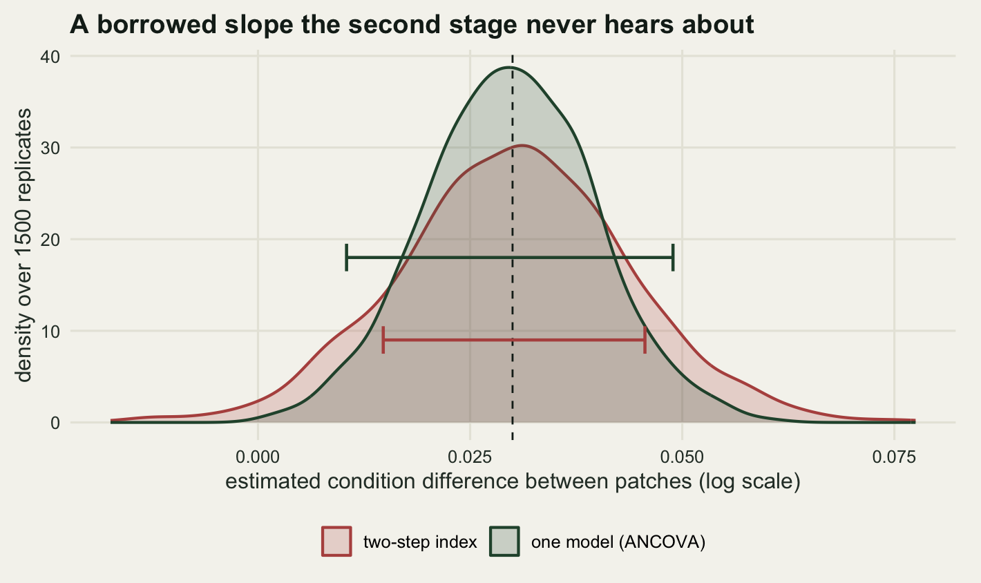
2.9946 0.2344 The two-step index is not biased. Over 1500 replicates it averages 0.03018 against a truth of 0.03, and the one-model analysis of covariance averages 0.02967. Both are doing the arithmetic right.
The intervals are a different story. The two-step reports a mean standard error of 0.00782 while its estimates vary across replicates with a standard deviation of 0.01353, a ratio of 1.7305; the one model reports 0.00975 against a spread of 0.00988, a ratio of 1.0124. Coverage follows: 75.67 per cent for the two-step against 94.2, and under a true null the two-step rejects in 25.53 per cent of replicates against the one model’s 5.2.
The missing variance has a closed-form approximation. The contrast is \((\bar{y}_1 - \bar{y}_0) - \hat{b}(\bar{x}_1 - \bar{x}_0)\), so it inherits \(\operatorname{Var}(\hat{b})\) multiplied by the squared difference in mean log tarsus between the patches. Relative to the variance the second stage does report, that extra term is \(n \Delta^2 / (4 m s_x^2)\) for a study of \(n\) birds split evenly, a reference series of \(m\), a between-patch gap \(\Delta\) and a within-patch tarsus spread \(s_x\). That predicts a variance ratio of 2.875 against a measured 2.9946.
Two things in that formula are worth carrying around. The damage grows with the square of how different the groups are in the nuisance variable, so a condition index is at its most dangerous exactly when the comparison is between groups that differ in size, which is usually the comparison somebody wants. And it grows with the study sample size: more study birds on the same borrowed exponent makes the interval narrower and the coverage worse, because the term the second stage reports shrinks and the term it omits stays where it is.
Carrying the first stage through
Suppose the condition index really is the quantity of interest rather than a nuisance adjustment. That is defensible: a scaled measure of mass at a given skeletal size is a biological estimand in its own right, and Peig and Green (2009) argue that the interesting version of it is not an ordinary least squares residual anyway. If the index is what gets reported, it cannot be replaced by putting tarsus in the model, because that answers a different question. The uncertainty has to be carried rather than dropped.
The way to do that is to resample the whole two-stage procedure. Each bootstrap replicate draws a new reference series with replacement, refits the exponent, draws a new study sample with replacement within each patch, recomputes every index with the resampled exponent, and takes the patch contrast. The interval is the percentile range of those contrasts, and nothing about the estimator changes.
i_p0 <- which(hab == 0)
i_p1 <- which(hab == 1)

boot_ci <- function(sv, n_boot) {
  vals <- numeric(n_boot)
  for (b in seq_len(n_boot)) {
    jr <- sample.int(m_ref, m_ref, replace = TRUE)
    j0 <- sample(i_p0, n_half, replace = TRUE)
    j1 <- sample(i_p1, n_half, replace = TRUE)
    bh <- slope1(sv$ltar_r[jr], sv$lmass_r[jr])
    vals[b] <- mean(sv$lmass_s[j1] - bh * sv$ltar_s[j1]) -
      mean(sv$lmass_s[j0] - bh * sv$ltar_s[j0])
  }
  unname(quantile(vals, c(0.025, 0.975)))
}

n_rep_b <- 500
n_boot <- 500

boot_run <- function(tau, seed) {
  set.seed(seed)
  t(replicate(n_rep_b, {
    sv <- sim_cond(tau)
    pf <- pair_fit(sv)
    c(pf[1], pf[2], pf[3], pf[4], boot_ci(sv, n_boot))
  }))
}

boot_alt <- boot_run(tau_true, 70401)
boot_nul <- boot_run(0, 70402)

boot_tab <- data.frame(
  method = c("two-step, printed interval", "one model (ANCOVA)",
             "two-step, bootstrapped"),
  coverage = c(mean(abs(boot_alt[, 1] - tau_true) < t_c2 * boot_alt[, 2]),
               mean(abs(boot_alt[, 3] - tau_true) < t_c3 * boot_alt[, 4]),
               mean(boot_alt[, 5] < tau_true & boot_alt[, 6] > tau_true)),
  width = c(mean(2 * t_c2 * boot_alt[, 2]),
            mean(2 * t_c3 * boot_alt[, 4]),
            mean(boot_alt[, 6] - boot_alt[, 5])),
  type_i = c(mean(abs(boot_nul[, 1] / boot_nul[, 2]) > t_c2),
             mean(abs(boot_nul[, 3] / boot_nul[, 4]) > t_c3),
             mean(!(boot_nul[, 5] < 0 & boot_nul[, 6] > 0))))
print(round(boot_tab[, -1], 5))
coverage width type_i
1 0.730 0.03092 0.230
2 0.958 0.03847 0.056
3 0.946 0.05243 0.062print(boot_tab$method)[1] "two-step, printed interval" "one model (ANCOVA)"
[3] "two-step, bootstrapped" print(round(c(boot_over_printed = boot_tab$width[3] / boot_tab$width[1],
boot_over_one_model = boot_tab$width[3] / boot_tab$width[2],
mc_se_coverage = sqrt(0.95 * 0.05 / n_rep_b)), 4)) boot_over_printed boot_over_one_model mc_se_coverage
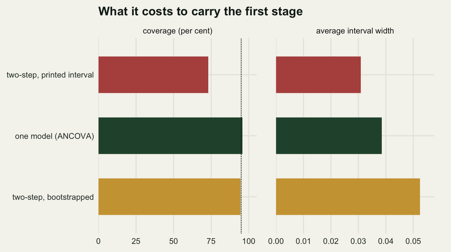
1.6958 1.3629 0.0097 Over 500 replicates with 500 bootstrap resamples each, the printed two-step interval covers 73 per cent of the time and rejects a true null in 23 per cent of replicates. Bootstrapping the whole procedure takes coverage to 94.6 per cent and the false-positive rate to 6.2 per cent. The Monte Carlo standard error on a coverage figure at this replicate count is 0.97 percentage points, so the bootstrap is at nominal within the resolution of the experiment and the printed interval is not.
The price is the width. The bootstrap interval averages 0.05243 against the printed interval’s 0.03092, a factor of 1.696. That factor is the finding restated: anything decided on the printed width was decided on an interval that needs to be 69.58 per cent wider.
A second comparison in that table decides the case for most analyses. The one model, fitting log mass on log tarsus and patch together using only the study birds, covers at 95.8 per cent with an interval of 0.03847, which is 26.63 per cent narrower than the bootstrapped two-step. Estimating the exponent from the study birds beats borrowing it and then paying to carry the borrowed uncertainty. The bootstrap is the right answer when the index itself is the deliverable, not when it is a way of avoiding a second term in a model.
Adjustment or definition
The five experiments separate into two cases that get treated as one, and the distinction decides what to do. In the first case the residual is an adjustment. Nobody wants to know about effort-corrected social strength as a biological quantity; they want the effect of social strength on fledging success holding effort constant, and residualising is a way of getting there. In that case the residual buys nothing. If the predictor is the residualised side, the estimate matches the one model’s to within floating-point error and the interval is 1.341 times too wide, costing 21.95 percentage points of power. If the response is the residualised side, the estimate is shrunk by 72.15 per cent at this correlation and coverage is 0.2 per cent. There is no version of the two-step that beats writing both variables into one model and accepting the standard error the collinearity earns.
In the second case the residual is a definition. A condition index is a claim about what mass at a given size means, and the number itself is reported, ranked, mapped and correlated with other things. A residualised diversity index used as a site-level attribute is the same kind of object. Here the two-step is not a shortcut around a model; it is the estimand, and the question is not whether to compute it but how to report its uncertainty. The answer measured above is that the second stage’s printed interval is wrong whenever the first stage was fitted somewhere else, by a factor of 1.696 in this setting, and that resampling both stages together brings coverage back from 73 to 94.6 per cent.
The test for which case you are in is one question. Would the residual still be interesting if the nuisance variable could be held constant by design? If a hypothetical study in which every bird had identical sighting effort would make it pointless, it was an adjustment, and it belongs in the model rather than in front of it. If it would still be the quantity of interest, because mass at a given size is what the biology is about, it is a definition, and the first stage is part of the estimator and has to be resampled with it.
The honest limit
Everything measured here lives inside a linear model with Gaussian errors, no measurement error in the nuisance variable, and a first stage that is either the same least squares projection the second stage would have applied or a slope estimated from an independent sample. Those two cases bracket a lot of practice but not all of it.
The gap that matters most is measurement error. Sighting effort is a count, and a count of sessions is a noisy proxy for the exposure that actually generates the association scores; tarsus is measured to a tenth of a millimetre by different people. When the nuisance variable carries error, neither the one model nor any residual route recovers the partial slope, because the quantity being held constant is not the quantity that matters. The one model is then biased too, and the comparison in this post, which is between an unbiased estimator and a shrunken one, becomes a comparison between two biased estimators whose ordering depends on the size of the error. Nothing measured above tells you which wins.
The second limit is the linear first stage. An allometric relationship fitted on the log scale is linear by construction, but a condition index built from a curved relationship, or one where the variance grows with size, produces residuals that are still correlated with the variable they were supposed to be free of. That correlation is easy to check and almost never checked: plot the index against the nuisance variable and look for structure. Peig and Green (2009) built their alternative index precisely because the ordinary residual keeps a dependence on size that its users assume is gone.
The third is that the shrinkage factor \(1 - R^2\) is exact only when the first stage is fitted on the same rows as the second. Computing an index once over a whole database and then analysing a subset of it, which is normal practice, sits between the two cases measured here, and where in between depends on a subset rule that is rarely written down.
Where to go next
The practical rule is short. If two predictors are correlated and you want the partial effect of one, fit both and report the wider interval; the sweep above shows it holding nominal coverage from a variance inflation factor of 1.33 to 10.26 while the two-step’s went from 73.7 per cent to 0. If the residual is the quantity you mean, keep it and bootstrap both stages, which cost 69.58 per cent in interval width here and bought back 21.6 percentage points of coverage.
For the diagnostics that start this argument, collinearity and VIF computes the variance inflation factor by hand and says what the thresholds are worth. Where the nuisance variable is sampling effort in a count model, offsets for rates and densities shows the version that needs no residual at all: log effort enters with its coefficient fixed at one, so the model is about rates and nothing has to be cleaned beforehand. And network centrality and sampling effort is where the residual route gets recommended on this blog; read it with the numbers above attached, noting that there the residualised variable is the predictor, the version that keeps the point estimate and spends power.
References
Frisch R, Waugh FV 1933 Econometrica 1(4):387 (10.2307/1907330)
Lovell MC 2008 The Journal of Economic Education 39(1):88-91 (10.3200/JECE.39.1.88-91)
Pagan A 1984 International Economic Review 25(1):221-247 (10.2307/2648877)
Garcia-Berthou E 2001 Journal of Animal Ecology 70(4):708-711 (10.1046/j.1365-2656.2001.00524.x)
Darlington RB, Smulders TV 2001 Animal Behaviour 62(3):599-602 (10.1006/anbe.2001.1806)
Freckleton RP 2002 Journal of Animal Ecology 71(3):542-545 (10.1046/j.1365-2656.2002.00618.x)
Peig J, Green AJ 2009 Oikos 118(12):1883-1891 (10.1111/j.1600-0706.2009.17643.x)