set.seed(1)
n <- 120
cover       <- runif(n, 0, 1)                                     # forest cover gradient, 0 to 1
trap_nights <- round(exp(1.9 + 0.9 * cover + rnorm(n, 0, 0.25)))  # effort rises with cover
trap_nights[trap_nights < 1] <- 1
b0 <- log(2)                                                      # true density: 2 beetles per night at cover 0
b1 <- -1.5                                                        # density declines with cover
log_density <- b0 + b1 * cover
mu          <- exp(log_density) * trap_nights                    # expected count = density times effort
count       <- rpois(n, mu)
dat <- data.frame(count, cover, trap_nights)Offsets for rates and densities in Poisson GLMs
R
GLM
count data
ecology tutorial
Sampling effort varies between sites and distorts raw counts. Add a log-effort offset to a Poisson GLM to model rates and densities, and recover the truth.
Counts almost never come from equal effort. One site was trapped for five nights, another for twenty-nine; one transect was four hundred metres, another was a kilometre; one quadrat was searched for ten minutes, another for half an hour. The raw count from each unit is a product of two things you care about separately: the underlying rate or density, and the amount of effort that went into observing it. Compare the raw counts directly and you are comparing density confounded with effort.
The fix is an offset. In a Poisson or negative binomial GLM you add the log of the effort as a model term whose coefficient is fixed at one, not estimated. That single line converts a model of counts into a model of rates, and it does so while keeping the count likelihood intact, which is exactly what you want and exactly what dividing by effort throws away.
This post builds a synthetic pitfall-trapping study where effort is tangled up with the very gradient under study, shows how the naive count model gets the answer wrong, and recovers the truth with an offset.
The trap: effort correlates with the predictor
A field reality that makes this more than a bookkeeping nicety: effort is often not random. Denser forest is harder to access, so you leave traps out longer; productive sites get more survey time because something is always happening there. When effort correlates with your predictor, ignoring it does not just add noise, it biases the slope.
Here, ground-beetle activity density truly declines with forest cover, but trap-nights rise with cover by construction, so the extra effort at high-cover sites props the raw counts up and flattens the apparent decline.
Before modelling, confirm the entanglement and look at the spread of effort.
round(cor(dat$cover, dat$trap_nights), 3) # effort tied to the predictor[1] 0.643range(dat$trap_nights) # effort varies five- to six-fold[1] 5 29range(dat$count)[1] 2 21Effort correlates with cover at 0.64, and trap-nights run from 5 to 29. That is a near six-fold range in observation effort across sites, structured along the gradient. The plot below is the heart of the problem.
library(ggplot2)
d1 <- data.frame(
  cover  = rep(dat$cover, 2),
  effort = rep(dat$trap_nights, 2),
  value  = c(dat$count, dat$count / dat$trap_nights),
  metric = rep(c("raw count", "density (count / trap-night)"), each = nrow(dat)))
d1$metric <- factor(d1$metric, levels = c("raw count", "density (count / trap-night)"))
ggplot(d1, aes(cover, value)) +
  geom_point(aes(size = effort), colour = "#275139", alpha = 0.55) +
  geom_smooth(method = "loess", formula = y ~ x, se = FALSE,
              colour = "#b5534e", linewidth = 0.9) +
  facet_wrap(~metric, scales = "free_y") +
  scale_size_continuous(range = c(0.6, 3.6), name = "trap-nights") +
  labs(x = "forest cover", y = NULL) +
  theme_minimal(base_size = 12) +
  theme(panel.grid.minor = element_blank(),
        strip.text = element_text(colour = "#16241d", face = "bold"),
        plot.background = element_rect(fill = "#f5f4ee", colour = NA),
        panel.background = element_rect(fill = "#f5f4ee", colour = NA))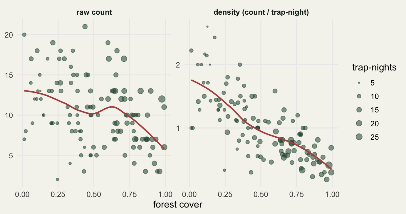
The left panel is what the naive model sees: a gently declining, noisy cloud. The right panel is the truth the offset will recover, a much steeper fall.
The naive model gets the slope wrong
Fit the obvious thing, count on cover, and read the slope.
m_naive <- glm(count ~ cover, family = poisson, data = dat)
round(summary(m_naive)$coefficients, 3)
Estimate Std. Error z value Pr(>|z|)
(Intercept) 2.628 0.057 46.127 0
cover -0.577 0.105 -5.495 0The slope on cover is about -0.58 and clearly significant, so you would report a real decline. The trouble is the number is wrong: the true effect on log-density is -1.5, and the naive model returns roughly a third of it. The rising effort has eaten much of the signal. A confident, significant, and badly biased estimate is worse than no estimate, because nothing in the output warns you.
The offset recovers the truth
Add offset(log(trap_nights)) to the formula. This says: the expected count is the density multiplied by effort, so on the log scale the log of effort enters with a coefficient of exactly one. Everything else in the linear predictor now describes the rate per trap-night.
m_off <- glm(count ~ cover + offset(log(trap_nights)),
             family = poisson, data = dat)
round(summary(m_off)$coefficients, 3)
Estimate Std. Error z value Pr(>|z|)
(Intercept) 0.664 0.057 11.656 0
cover -1.416 0.105 -13.496 0c(true_intercept = round(b0, 3), true_slope = b1)true_intercept true_slope
0.693 -1.500 Now the slope on cover is -1.42 against a true -1.5, and the intercept is 0.66 against a true 0.69. The model has separated density from effort and landed on the real gradient. The standard error is essentially unchanged from the naive fit; the offset corrects the bias, it does not cost precision.
ci_n <- confint(m_naive)["cover", ]; est_n <- coef(m_naive)["cover"]Waiting for profiling to be done...ci_o <- confint(m_off)["cover", ]; est_o <- coef(m_off)["cover"]Waiting for profiling to be done...fd <- data.frame(
model = factor(c("naive (count ~ cover)", "offset (rate ~ cover)"),
levels = c("offset (rate ~ cover)", "naive (count ~ cover)")),
est = c(est_n, est_o), lo = c(ci_n[1], ci_o[1]), hi = c(ci_n[2], ci_o[2]))
ggplot(fd, aes(est, model)) +
geom_vline(xintercept = b1, linetype = "dashed", colour = "#93a87f", linewidth = 0.7) +
geom_errorbarh(aes(xmin = lo, xmax = hi), height = 0.16, colour = "#275139", linewidth = 0.9) +
geom_point(size = 3.4, colour = "#275139") +
annotate("text", x = b1, y = 2.42, label = "true slope = -1.5",
colour = "#46604a", size = 3.3, family = "mono", hjust = 0.5) +
scale_x_continuous(expand = expansion(mult = c(0.08, 0.05))) +
labs(x = "cover slope (95% CI)", y = NULL) +
theme_minimal(base_size = 12) +
theme(panel.grid.minor = element_blank(),
plot.background = element_rect(fill = "#f5f4ee", colour = NA),
panel.background = element_rect(fill = "#f5f4ee", colour = NA))Warning: `geom_errorbarh()` was deprecated in ggplot2 4.0.0.
ℹ Please use the `orientation` argument of `geom_errorbar()` instead.`height` was translated to `width`.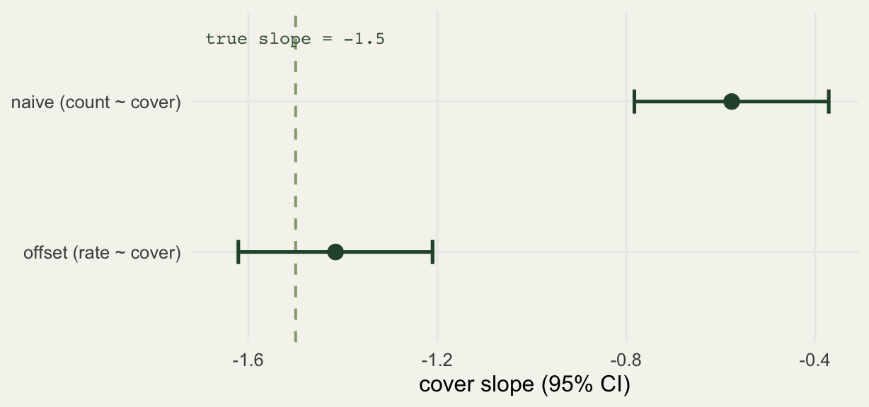
Reading predictions as densities
Because the offset model is on a per-effort scale, you can read predictions directly as densities by setting effort to one. With trap_nights = 1 the offset term is log(1) = 0, so the prediction is the rate itself.
nd <- data.frame(cover = c(0, 1), trap_nights = 1)
pred <- predict(m_off, newdata = nd, type = "response")
round(pred, 3)                                  # density per trap-night at cover 0 and 1
1 2
1.942 0.472 round(c(true_0 = exp(b0), true_1 = exp(b0 + b1)), 3)true_0 true_1
2.000 0.446 The model predicts 1.94 beetles per trap-night at zero cover and 0.47 at full cover, against true densities of 2.0 and 0.45. Plotted across the gradient, the fitted density curve tracks the truth, and the observed rates scatter around it with the high-effort points sitting closer in, which is the precision the offset preserves and the ratio approach discards.
grid <- data.frame(cover = seq(0, 1, length.out = 100), trap_nights = 1)
pr <- predict(m_off, newdata = grid, type = "link", se.fit = TRUE)
grid$fit <- exp(pr$fit)
grid$lo  <- exp(pr$fit - 1.96 * pr$se.fit)
grid$hi  <- exp(pr$fit + 1.96 * pr$se.fit)
grid$tru <- exp(b0 + b1 * grid$cover)
obs <- data.frame(cover = dat$cover, rate = dat$count / dat$trap_nights,
                  effort = dat$trap_nights)
ggplot() +
  geom_ribbon(data = grid, aes(cover, ymin = lo, ymax = hi),
              fill = "#275139", alpha = 0.16) +
  geom_point(data = obs, aes(cover, rate, size = effort),
             colour = "#46604a", alpha = 0.5) +
  geom_line(data = grid, aes(cover, fit), colour = "#275139", linewidth = 1) +
  geom_line(data = grid, aes(cover, tru), colour = "#b5534e",
            linetype = "dashed", linewidth = 0.8) +
  scale_size_continuous(range = c(0.6, 3.6), name = "trap-nights") +
  labs(x = "forest cover", y = "density (beetles per trap-night)") +
  theme_minimal(base_size = 12) +
  theme(panel.grid.minor = element_blank(),
        plot.background = element_rect(fill = "#f5f4ee", colour = NA),
        panel.background = element_rect(fill = "#f5f4ee", colour = NA))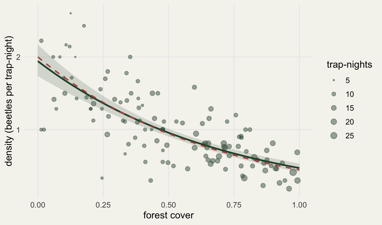
Why not just model count divided by effort?
The obvious shortcut is to compute a rate, count / trap_nights, and put that on the left of an ordinary linear model. It is tempting and it is wrong, for two reasons.
First, it breaks the variance structure. A Poisson count has variance equal to its mean, so a count of 20 carries more information than a count of 2. Once you divide by effort and hand the ratio to a Gaussian model, every site is treated as equally precise, regardless of whether it rests on 5 trap-nights or 29. You have thrown away the fact that the high-effort sites pin the rate down far more tightly. The offset keeps the count as the response, so the likelihood still weights each observation by its true precision.
Second, ratios are awkwardly distributed: bounded below by zero, skewed, and heteroscedastic in exactly the way a linear model assumes away. A small count over a small effort produces a noisy, lumpy ratio that no amount of transformation fully tames. Modelling the count with an offset sidesteps the whole problem because you never form the ratio at all.
Overdispersion and the negative binomial
Check that the Poisson assumption holds by comparing residual deviance to its degrees of freedom.
round(deviance(m_off) / df.residual(m_off), 3)[1] 1.098Here the ratio is about 1.1, comfortably close to one, so Poisson is fine. Real count data are frequently overdispersed (the ratio runs well above one), in which case the standard errors from a Poisson fit are too small and the offset alone will not save you. The remedy is to keep the offset and switch the family: MASS::glm.nb(count ~ cover + offset(log(trap_nights))) fits a negative binomial with the identical offset logic. The offset is orthogonal to the choice of count distribution; it addresses effort, the family addresses dispersion, and you fix both at once.
Practical guidance
A handful of rules that travel well:
Use an offset whenever your units differ in size, duration, area, or effort, and you want a rate or a density rather than a raw tally. Transect length, trap-nights, person-hours, plot area, and search time are all offsets; the variable goes in as offset(log(effort)), always logged, because the link is logarithmic.
The offset coefficient is fixed, not fitted. If you instead add log(effort) as an ordinary predictor, you let the model estimate its slope, which answers a different question (does effort have a non-proportional effect) and no longer gives you a clean rate. Reserve that only when you genuinely doubt proportionality.
Log the effort, not the response. The offset enters on the scale of the linear predictor, which for Poisson and negative binomial is the log scale, so it is offset(log(trap_nights)), never offset(trap_nights).
Predict at effort one to read densities directly, as above, or at a realistic effort to predict actual counts. Both are valid; just be clear which scale you are reporting.
The deeper point, which O’Hara and Kotze argue forcefully, is to model counts as counts rather than mangling them into ratios or logs of the response. The offset is how you respect both the count nature of the data and the unequal effort behind it, in one term.
References
O’Hara and Kotze 2010 Methods in Ecology and Evolution 1(2):118-122 (10.1111/j.2041-210X.2010.00021.x)
Zuur, Ieno, Walker, Saveliev and Smith 2009 Mixed Effects Models and Extensions in Ecology with R, Springer (ISBN 978-0-387-87457-9)
Kery 2010 Introduction to WinBUGS for Ecologists, Academic Press (ISBN 978-0-12-378605-0)