---
title: "Dispersion checks when the counts are small"
description: "Residual deviance over degrees of freedom is the standard overdispersion check, and on ecological count sizes it fails in both directions. Measured in R."
date: "2026-08-07 09:00"
categories: [R, GLM, count data, model checking, ecology tutorial]
image: thumbnail.png
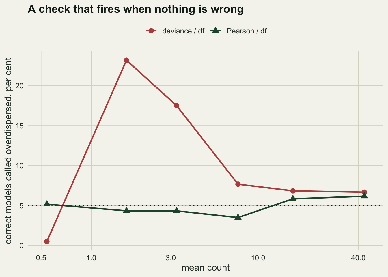
image-alt: "Rejection rate of two dispersion statistics against mean count, with the deviance curve starting below the nominal five per cent line at the smallest mean count, then peaking far above it and remaining above it across the rest of the range, while the Pearson curve stays close to it."
---
Fit a Poisson GLM and the next line is almost always the same one: divide the residual deviance by its degrees of freedom and see whether the answer is near one. It is in the textbooks, it is in the teaching material, and it appears on this site in the posts on [GLMs for count data](../glm-count-data-abundance/) and [offsets for rates and densities](../offsets-for-rates-and-densities/). The habit is sound. The statistic is the problem.
There are two statistics in general use for this, and they are usually printed side by side without comment. One of them holds its nominal error rate across every count size an ecologist is likely to have. The other does not, and the sizes where it goes wrong are exactly the sizes that ecological counts come in: a handful of beetles per trap, a few seedlings per quadrat, one or two detections per visit.
This post fits correctly specified models, so every rejection is a false alarm by construction, and measures how often each check raises one.
## The check, and the two statistics behind it
Both statistics measure the same thing, the total discrepancy between observed counts and fitted means, and both are compared with a chi-squared distribution on the residual degrees of freedom. They differ in how they weight a discrepancy. The deviance is twice the log-likelihood gap between the fitted model and a model that fits every observation exactly. The Pearson statistic is the sum of squared Pearson residuals, each observation's departure divided by its own standard deviation.
```{r setup}
#| message: false
#| warning: false
library(ggplot2)
suppressMessages(library(MASS))

te_paper  <- "#f5f4ee"
te_ink    <- "#16241d"
te_body   <- "#2c3a31"
te_forest <- "#275139"
te_rust   <- "#b5534e"
te_gold   <- "#c9b458"
te_line   <- "#dad9ca"

theme_datasheet <- function() {
  theme_minimal(base_size = 12) +
    theme(plot.background  = element_rect(fill = te_paper, colour = NA),
          panel.background = element_rect(fill = te_paper, colour = NA),
          panel.grid.major = element_line(colour = te_line, linewidth = 0.3),
          panel.grid.minor = element_blank(),
          text             = element_text(colour = te_body),
          plot.title       = element_text(colour = te_ink, face = "bold"),
          axis.text        = element_text(colour = te_body))
}

# one correctly specified Poisson data set, both statistics and both p values
one_fit <- function(n, mu0, slope = 0.4) {
  x <- rnorm(n)
  y <- rpois(n, exp(log(mu0) + slope * x))
  m <- glm(y ~ x, family = poisson)
  dfr <- df.residual(m)
  pear <- sum(residuals(m, type = "pearson")^2)
  c(mean_count = mean(y),
    dev_ratio  = deviance(m) / dfr,
    pear_ratio = pear / dfr,
    p_dev      = pchisq(deviance(m), dfr, lower.tail = FALSE),
    p_pear     = pchisq(pear, dfr, lower.tail = FALSE))
}

set.seed(4041)
example <- one_fit(120, 1.5)
round(example, 4)
```
On that single dataset, generated from an exactly Poisson process, the deviance ratio is `r sprintf("%.3f", example[["dev_ratio"]])` and the Pearson ratio `r sprintf("%.3f", example[["pear_ratio"]])`. A reader following the usual rule would look at the first number and start worrying about overdispersion that is not there.
## Six count sizes, all correctly specified
One dataset proves nothing, so repeat it across a range of mean counts. The model is right every time, so the correct rejection rate is five per cent everywhere.
```{r size}
mu_grid <- c(0.5, 1.5, 3, 7, 15, 40)
n_rep <- 600

set.seed(909)
size <- do.call(rbind, lapply(mu_grid, function(mu) {
  r <- t(replicate(n_rep, one_fit(120, mu)))
  data.frame(mean_count = mean(r[, "mean_count"]),
             dev_ratio  = mean(r[, "dev_ratio"]),
             pear_ratio = mean(r[, "pear_ratio"]),
             rej_dev    = 100 * mean(r[, "p_dev"]  < 0.05),
             rej_pear   = 100 * mean(r[, "p_pear"] < 0.05))
}))
round(size, 3)
```
The Pearson column does what a test is supposed to do: `r sprintf("%.1f", min(size$rej_pear))` to `r sprintf("%.1f", max(size$rej_pear))` per cent across the whole range, which is five per cent give or take simulation noise. The deviance column peaks at `r sprintf("%.1f", max(size$rej_dev))` per cent, at a mean count of `r sprintf("%.1f", size$mean_count[which.max(size$rej_dev)])`, and does not settle down to the nominal rate until the counts are into the teens.
The failure is not monotone, which is worth pausing on, because it means there is no simple rule of the form "trust it above such and such a count". At the lowest mean the deviance test rejects only `r sprintf("%.1f", size$rej_dev[1])` per cent of the time, so it has become conservative rather than liberal. In between it is badly liberal. The reason is that the chi-squared approximation to the deviance is an approximation in the number of observations only when each observation carries enough information, and a count of zero or one carries very little; with means below one the deviance is dominated by a discrete lump of possible values and its distribution is nothing like a chi-squared.
```{r fig-size}
#| fig-cap: "False alarm rate of each dispersion check against mean count, on data generated from a correctly specified Poisson model. Six hundred simulated datasets of 120 observations per point; the dotted line is the nominal five per cent."
#| fig-alt: "Two curves against mean count on a logarithmic axis. The deviance curve starts near zero, rises to about twenty three per cent at a mean count near one and a half, then falls slowly towards five as the counts grow. The Pearson curve stays flat along the five per cent line throughout."
long <- rbind(data.frame(mu = size$mean_count, y = size$rej_dev,
                         stat = "deviance / df"),
              data.frame(mu = size$mean_count, y = size$rej_pear,
                         stat = "Pearson / df"))

ggplot(long, aes(mu, y, colour = stat, shape = stat)) +
  geom_hline(yintercept = 5, linetype = "dotted", colour = te_ink,
             linewidth = 0.6) +
  geom_line(linewidth = 0.9) +
  geom_point(size = 2.9) +
  scale_x_log10(breaks = c(0.5, 1, 3, 10, 40), expand = expansion(mult = 0.06)) +
  scale_colour_manual(values = c("deviance / df" = te_rust,
                                 "Pearson / df" = te_forest)) +
  scale_shape_manual(values = c(16, 17)) +
  labs(x = "mean count", y = "correct models called overdispersed, per cent",
       colour = NULL, shape = NULL,
       title = "A check that fires when nothing is wrong") +
  theme_datasheet() +
  theme(legend.position = "top")
```
The ratios themselves tell the same story more quietly. The deviance ratio averages `r sprintf("%.3f", size$dev_ratio[which.max(size$rej_dev)])` at the worst count size, which is the kind of number that looks like mild overdispersion and gets reported as such, while the Pearson ratio sits at `r sprintf("%.3f", size$pear_ratio[which.max(size$rej_dev)])`.
## Binary data breaks it completely
Presence and absence data is the extreme case, and here the deviance check is not approximately wrong, it is structurally meaningless. For ungrouped binary responses the deviance depends only on the fitted probabilities, not on the observed zeros and ones at all, so it cannot carry information about how well those fitted probabilities match the data.
```{r binary}
one_binary <- function(n) {
  x <- rnorm(n)
  y <- rbinom(n, 1, plogis(0.2 + 0.8 * x))
  m <- glm(y ~ x, family = binomial)
  c(ratio = deviance(m) / df.residual(m),
    p     = pchisq(deviance(m), df.residual(m), lower.tail = FALSE))
}

set.seed(515)
binary <- do.call(rbind, lapply(c(100, 400, 1600), function(n) {
  r <- t(replicate(400, one_binary(n)))
  data.frame(n = n, dev_ratio = mean(r[, "ratio"]),
             rejects = 100 * mean(r[, "p"] < 0.05))
}))
round(binary, 3)
```
Every one of these models is correctly specified. At `r binary$n[1]` observations the test rejects `r sprintf("%.1f", binary$rejects[1])` per cent of them, and at `r binary$n[3]` it rejects `r sprintf("%.1f", binary$rejects[3])` per cent. The check gets worse with more data, which is the clearest possible sign that it is not a test of anything.
Grouping the observations first is the standard repair: sort by fitted probability, cut into bins, and compare observed with expected counts within bins.
```{r grouped}
grouped_p <- function(n, k) {
  x <- rnorm(n); y <- rbinom(n, 1, plogis(0.2 + 0.8 * x))
  m <- glm(y ~ x, family = binomial); fv <- fitted(m)
  g  <- cut(rank(fv, ties.method = "first"), breaks = k, labels = FALSE)
  o  <- tapply(y,  g, sum)
  e  <- tapply(fv, g, sum)
  sz <- tapply(y,  g, length)
  pchisq(sum((o - e)^2 / (e * (1 - e / sz))), k - 2, lower.tail = FALSE)
}

set.seed(77)
grouped <- do.call(rbind, lapply(c(8, 20, 50), function(k) {
  data.frame(bins = k,
             rejects = 100 * mean(replicate(400, grouped_p(400, k)) < 0.05))
}))
round(grouped, 2)
```
With the same 400 observations, grouping brings the rate back to between `r sprintf("%.1f", min(grouped$rejects))` and `r sprintf("%.1f", max(grouped$rejects))` per cent at every bin count tried, against `r sprintf("%.1f", binary$rejects[2])` per cent for the ungrouped deviance.
## The same check also misses real overdispersion
A test that raises false alarms might at least be sensitive. At the smallest counts the deviance check manages neither.
```{r power}
one_nb <- function(n, mu0, theta = 2, slope = 0.4) {
  x <- rnorm(n)
  y <- rnegbin(n, exp(log(mu0) + slope * x), theta)
  m <- glm(y ~ x, family = poisson); dfr <- df.residual(m)
  c(p_dev  = pchisq(deviance(m), dfr, lower.tail = FALSE),
    p_pear = pchisq(sum(residuals(m, type = "pearson")^2), dfr,
                    lower.tail = FALSE))
}

set.seed(313)
power <- do.call(rbind, lapply(c(0.5, 1.5, 3, 7), function(mu) {
  r <- t(replicate(500, one_nb(120, mu)))
  data.frame(mu = mu, power_dev = 100 * mean(r[, "p_dev"] < 0.05),
             power_pear = 100 * mean(r[, "p_pear"] < 0.05))
}))
round(power, 1)
```
The data is now genuinely overdispersed, drawn from a negative binomial with a shape parameter of 2, which is severe. At a mean count of `r sprintf("%.1f", power$mu[1])` the deviance check finds it in `r sprintf("%.1f", power$power_dev[1])` per cent of datasets while the Pearson check finds it in `r sprintf("%.1f", power$power_pear[1])` per cent. From a mean of `r sprintf("%.1f", power$mu[2])` upwards both are at or near `r sprintf("%.0f", 100)` per cent, so the disagreement is confined to the sparse end, but the sparse end is where zero-heavy ecological counts live.
## The general repair, when you do not trust either approximation
Both statistics are being compared with a reference distribution that is an approximation. The approximation can be replaced with the real thing by simulating from the fitted model.
```{r bootstrap}
boot_dev <- function(n, mu0, B = 199, slope = 0.4) {
  x <- rnorm(n); y <- rpois(n, exp(log(mu0) + slope * x))
  m <- glm(y ~ x, family = poisson)
  d0 <- deviance(m); fv <- fitted(m)
  ds <- replicate(B, deviance(glm(rpois(n, fv) ~ x, family = poisson)))
  (1 + sum(ds >= d0)) / (1 + B)
}

set.seed(6262)
boot_rate <- 100 * mean(replicate(200, boot_dev(120, 1.5)) < 0.05)
boot_rate
```
At the count size where the chi-squared reference gave `r sprintf("%.1f", size$rej_dev[2])` per cent, the parametric bootstrap gives `r sprintf("%.1f", boot_rate)` per cent. The statistic was never the problem; the distribution it was compared against was.
## What to report
If you are going to quote one number, quote the Pearson ratio, and say which one it is. The two ratios are printed in the same summary and differ by enough at small counts to change the conclusion, so "the dispersion statistic was 1.13" is not a reproducible sentence.
Do not report a deviance goodness-of-fit test for a binary response. There is no count size at which it becomes valid, because the problem is not the sample size.
State the mean count alongside the dispersion statistic. It is one number, it costs nothing, and it lets a reader work out whether the approximation behind the check was in a range where it holds.
For anything beyond a single scalar, simulation-based quantile residuals give a diagnostic that works at any count size and shows the shape of the misfit rather than its total, and the post on [GLM residual diagnostics](../glm-residual-diagnostics/) builds them from scratch.
## Honest limits
Everything above uses one predictor, 120 observations and a single slope. The residual degrees of freedom, the number of parameters and the spread of the fitted means all move the approximation, and a model with many parameters relative to observations behaves worse than this one. The direction of the failure carries over; the exact rates do not.
The Pearson statistic is better calibrated here, not universally safe. Its own chi-squared approximation leans on the fitted means being reasonably large, and it is sensitive to a single observation with a small fitted mean and a large count, which is precisely the kind of point an ecological dataset contains. Its good behaviour in this simulation comes from the fitted means being smooth and the sample size being moderate.
A dispersion check of either kind answers a single yes or no about total discrepancy. It cannot distinguish overdispersion from a missing covariate, a wrong link, or zero inflation, and all three of those produce a ratio above one. Treating the ratio as a diagnosis rather than a symptom is a separate mistake from the one measured here.
The grouped test for binary data inherits the arbitrariness of the grouping. The rate was near nominal at every bin count tried above, but the statistic itself changes with the bins, and two analysts with different bin counts can report different p values for the same model.
Finally, the negative binomial used for the power section is one alternative among many. Overdispersion from clustering, from an omitted spatial term, or from a zero-generating process has a different signature, and a check tuned to one of them is not automatically sensitive to the others.
## References
Cox DR 1983 Biometrika 70(1):269-274 (10.1093/biomet/70.1.269)
Hosmer DW, Lemesbow S 1980 Communications in Statistics Theory and Methods 9(10):1043-1069 (10.1080/03610928008827941)
Dunn PK, Smyth GK 1996 Journal of Computational and Graphical Statistics 5(3):236-244 (10.1080/10618600.1996.10474708)
Ver Hoef JM, Boveng PL 2007 Ecology 88(11):2766-2772 (10.1890/07-0043.1)
## Related tutorials
- [GLM residual diagnostics](../glm-residual-diagnostics/)
- [Detecting a die-off from carcass reports](../detecting-a-die-off-from-carcass-reports/)
- [Taylor's power law and how many quadrats](../taylors-power-law-and-sample-size/)
- [Sequential sampling for pest decisions](../sequential-sampling-for-pest-decisions/)