library(ggplot2)

te_paper  <- "#f5f4ee"
te_ink    <- "#16241d"
te_body   <- "#2c3a31"
te_forest <- "#275139"
te_rust   <- "#b5534e"
te_gold   <- "#c9b458"
te_line   <- "#dad9ca"

theme_datasheet <- function() {
  theme_minimal(base_size = 12) +
    theme(plot.background  = element_rect(fill = te_paper, colour = NA),
          panel.background = element_rect(fill = te_paper, colour = NA),
          panel.grid.major = element_line(colour = te_line, linewidth = 0.3),
          panel.grid.minor = element_blank(),
          text             = element_text(colour = te_body),
          plot.title       = element_text(colour = te_ink, face = "bold"),
          plot.subtitle    = element_text(colour = te_body),
          axis.text        = element_text(colour = te_body),
          strip.text       = element_text(colour = te_ink))
}Sequential sampling for pest decisions
R
sampling
count data
decision analysis
simulation
ecology tutorial
A Wald sequential plan decides whether to spray after every plant, but its boundaries contain the negative binomial k. Checking the plan by simulation in R.
An adviser walks into a field of winter wheat in late spring with a hand lens and a clipboard. The question is not how many aphids there are. It is whether the field needs spraying, and the action threshold written in the regional guidance is a mean of three aphids per tiller. Below two the field is clearly safe, above four it clearly needs treatment, and between them the adviser would accept either answer. Counting a hundred tillers to estimate the mean precisely wastes the morning on fields that are obviously clean or obviously infested. What the adviser wants is a rule that says, after every tiller, whether to stop and decide or to keep counting.
That rule is Wald’s sequential probability ratio test, and it has been the backbone of pest sampling plans since the 1950s. The running total of insects is plotted against the number of plants examined, two parallel lines are drawn on the chart, and sampling stops the first time the total crosses one of them. Crossing the upper line means treat, crossing the lower line means do not.
The blog already has two neighbouring pieces of this machinery. Taylor’s power law and how many quadrats turns a variance to mean relationship into a sample size fixed in advance, with no stopping rule; testing a monitoring series every year spends a false alarm budget over annual looks at a trend test, which is sequential in years but not unit by unit. This post is the plant by plant plan. Its price, which the rest of the post measures, is that the aggregation parameter of the negative binomial sits inside the two lines, so a plan drawn with the wrong k is a different plan from the one its error rates were promised for. The same wrong k is also given to the fixed sample alternative, because a comparison that lets only the sequential plan be wrong would not be a comparison.
Two lines from a likelihood ratio
The plan tests a mean of m0 against a mean of m1 with the probability of treating a safe field held to alpha and the probability of leaving an infested field untreated held to beta. Wald (1945) showed that the log likelihood ratio, summed plant by plant, should be compared against two constants, log((1 - beta) / alpha) above and log(beta / (1 - alpha)) below. For negative binomial counts with a common k, the log likelihood ratio of one plant with count x is a straight line in x, so the sum over n plants is a straight line in the running total T. Rearranged for T, the two stopping boundaries are parallel lines with a common slope and intercepts of opposite sign. The review by Binns and Nyrop (1992) sets out the same lines for pest sampling; nothing below uses a table.
All design constants are fixed here, before any simulation: a safe mean of 2 and an infested mean of 4 per plant, both error rates at one tenth, an assumed k of 2, and a hard cap of 60 plants. If the cap is reached without a crossing, the field is treated when the running total lies above the midline between the two boundaries, which is the sign of the log likelihood ratio.
m0 <- 2
m1 <- 4
alpha_err <- 0.10
beta_err  <- 0.10
k_assumed <- 2
n_max     <- 60

a_up <- log((1 - beta_err) / alpha_err)
b_lo <- log(beta_err / (1 - alpha_err))

llr_coef <- function(k_plan) log(m1 * (k_plan + m0) / (m0 * (k_plan + m1)))
slope_of <- function(k_plan) k_plan * log((k_plan + m1) / (k_plan + m0)) / llr_coef(k_plan)

h_upper <- a_up / llr_coef(k_assumed)
h_lower <- b_lo / llr_coef(k_assumed)
s_slope <- slope_of(k_assumed)

set.seed(5207)
x_check   <- rnbinom(25, size = k_assumed, mu = 3)
llr_exact <- cumsum(dnbinom(x_check, size = k_assumed, mu = m1, log = TRUE) -
                    dnbinom(x_check, size = k_assumed, mu = m0, log = TRUE))
llr_line  <- llr_coef(k_assumed) * (cumsum(x_check) - s_slope * seq_along(x_check))
llr_gap   <- max(abs(llr_exact - llr_line))

h_upper_k05 <- a_up / llr_coef(0.5)
s_slope_k05 <- slope_of(0.5)
With k at 2 the upper boundary is T = 7.64 + 2.819 n and the lower one is T = -7.64 + 2.819 n. The slope, 2.819 insects per plant, sits between the two means and a little below their midpoint of 3, which is the negative binomial’s version of the Poisson slope. The line form was checked against the log likelihood ratio computed directly from dnbinom() on 25 simulated counts; the largest difference along the running sum is 9.21e-15, which is rounding.
The lines depend on k. Redrawn for a k of 0.5, the upper intercept is 20.85 and the slope 2.789. A more aggregated pest needs a much wider corridor, because single plants carry less information about the field mean when most of the insects sit on a few of them.
walk_one <- function(m, id) {
  x_w  <- rnbinom(n_max, size = k_assumed, mu = m)
  tot  <- cumsum(x_w)
  dev  <- tot - s_slope * seq_len(n_max)
  hit  <- which(dev >= h_upper | dev <= h_lower)[1]
  if (is.na(hit)) hit <- n_max
  data.frame(plant = 0:hit, total = c(0, tot[seq_len(hit)]),
             field = id, true_mean = paste("true mean", m))
}
set.seed(3118)
walk_df <- do.call(rbind, c(lapply(1:6, function(i) walk_one(m0, paste0("a", i))),
                            lapply(1:6, function(i) walk_one(m1, paste0("b", i)))))
walk_end <- do.call(rbind, lapply(split(walk_df, walk_df$field), function(d) d[nrow(d), ]))
n_show   <- max(walk_df$plant) + 2
line_df  <- data.frame(plant = c(0, n_show))

ggplot(walk_df, aes(plant, total)) +
  geom_ribbon(data = line_df, aes(x = plant, ymin = pmax(h_lower + s_slope * plant, 0),
                                  ymax = h_upper + s_slope * plant),
              inherit.aes = FALSE, fill = te_line, alpha = 0.6) +
  geom_abline(intercept = h_upper, slope = s_slope, colour = te_rust, linewidth = 0.8) +
  geom_abline(intercept = h_lower, slope = s_slope, colour = te_forest, linewidth = 0.8) +
  geom_step(aes(group = field, colour = true_mean), linewidth = 0.6) +
  geom_point(data = walk_end, aes(colour = true_mean), size = 2) +
  scale_colour_manual(values = c(te_forest, te_rust), name = NULL) +
  coord_cartesian(xlim = c(0, n_show), ylim = c(0, NA)) +
  labs(x = "plants examined", y = "running total of insects",
       title = "Stop at the first crossing",
       subtitle = "red line: treat; green line: do not treat; grey band: keep counting") +
  theme_datasheet() +
  theme(legend.position = "bottom")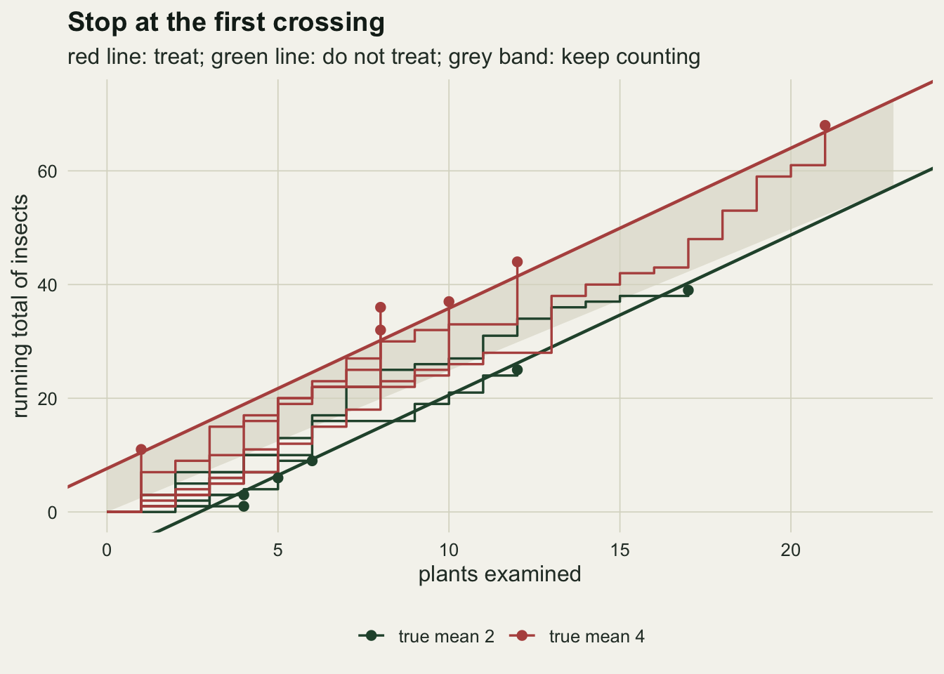
When k is right, the plan beats its own promise and Wald’s arithmetic misses
The plan is evaluated by simulation over a grid of true field means from 1 to 6, with 4000 simulated fields per cell. The whole walk of 60 plants is drawn at once for every field and the first crossing is found with max.col(), so the grid of five aggregation scenarios runs in a few seconds. The two quantities a sampling plan is judged by are the operating characteristic, here written as the probability of treating at each true mean, and the average sample number.
Wald also gave closed form approximations for both. The operating characteristic comes from the non-zero root h of E[exp(h z)] = 1, where z is the per plant log likelihood ratio increment and the expectation is taken under the TRUE count distribution, not under the one the plan assumed. For negative binomial counts that expectation is the negative binomial moment generating function, so the root is a one-dimensional uniroot(). The average sample number is then the expected log likelihood ratio at stopping divided by the expected increment. Both approximations pretend that the walk stops exactly on a boundary.
run_plan <- function(m, k_true, n_run, k_plan = k_assumed) {
  h_up <- a_up / llr_coef(k_plan)
  h_lo <- b_lo / llr_coef(k_plan)
  slp  <- slope_of(k_plan)
  counts <- matrix(rnbinom(n_run * n_max, size = k_true, mu = m), n_run)
  dev    <- t(apply(counts, 1, cumsum)) -
            matrix(slp * seq_len(n_max), n_run, n_max, byrow = TRUE)
  up_hit <- dev >= h_up
  lo_hit <- dev <= h_lo
  first_up <- ifelse(rowSums(up_hit) > 0, max.col(up_hit, "first"), n_max + 1)
  first_lo <- ifelse(rowSums(lo_hit) > 0, max.col(lo_hit, "first"), n_max + 1)
  capped   <- first_up > n_max & first_lo > n_max
  stop_n   <- pmin(first_up, first_lo, n_max)
  treat    <- ifelse(capped, dev[, n_max] > 0, first_up < first_lo)
  c(p_treat = mean(treat), asn = mean(stop_n),
    asn_se = sd(stop_n) / sqrt(n_run), capped = mean(capped))
}

wald_approx <- function(m, k_true, k_plan = k_assumed) {
  cf   <- llr_coef(k_plan)
  cc   <- cf * slope_of(k_plan)
  ez   <- cf * m - cc
  mgf1 <- function(h) (1 + m * (1 - exp(h * cf)) / k_true)^(-k_true) * exp(-h * cc) - 1
  h_cap <- log(1 + k_true / m) / cf
  h_root <- if (ez < 0) uniroot(mgf1, c(1e-6, h_cap * (1 - 1e-9)))$root else
                        uniroot(mgf1, c(-50, -1e-6))$root
  p_no  <- (exp(h_root * a_up) - 1) / (exp(h_root * a_up) - exp(h_root * b_lo))
  p_tr  <- 1 - p_no
  c(p_treat = p_tr, asn = (p_tr * a_up + (1 - p_tr) * b_lo) / ez)
}

n_run  <- 4000
m_grid <- seq(1, 6, by = 0.5)
k_grid <- c(4, 2, 1, 0.5)
taylor_a <- 2
taylor_b <- 1.5
k_taylor <- function(m) m^2 / (taylor_a * m^taylor_b - m)

scen <- rbind(expand.grid(m = m_grid, scenario = paste("k =", k_grid),
                          stringsAsFactors = FALSE),
              data.frame(m = m_grid, scenario = "Taylor law"))
is_taylor   <- scen$scenario == "Taylor law"
scen$k_true <- k_taylor(scen$m)
scen$k_true[!is_taylor] <- as.numeric(sub("k = ", "", scen$scenario[!is_taylor]))

set.seed(8841)
sim_tab  <- t(mapply(run_plan, scen$m, scen$k_true, MoreArgs = list(n_run = n_run)))
wald_tab <- t(mapply(wald_approx, scen$m, scen$k_true))
res <- cbind(scen, as.data.frame(sim_tab),
             wald_treat = wald_tab[, "p_treat"], wald_asn = wald_tab[, "asn"])
res$asn_miss <- (res$asn - res$wald_asn) / res$asn

pick <- function(sc, m) res[res$scenario == sc & res$m == m, ]
r2_0 <- pick("k = 2", m0);  r2_1 <- pick("k = 2", m1);  r2_mid <- pick("k = 2", 3)
r05_0 <- pick("k = 0.5", m0); r05_1 <- pick("k = 0.5", m1); r05_mid <- pick("k = 0.5", 3)
mc_se_err <- sqrt(0.1 * 0.9 / n_run)
miss_right <- range(res$asn_miss[res$scenario == "k = 2" & res$m %in% c(m0, 3, m1)])
miss_wrong <- range(res$asn_miss[res$scenario == "k = 0.5" & res$m %in% c(m0, 3, m1)])
cap_max <- max(res$capped)
miss_all <- range(res$asn_miss)
r1_0 <- pick("k = 1", m0); r1_1 <- pick("k = 1", m1)
With k really at 2, the plan treats a safe field (true mean 2) in 0.050 of runs and leaves an infested field (true mean 4) untreated in 0.087, against nominal rates of 0.10 each; the Monte Carlo standard error on a rate near one tenth is 0.0047. The average sample numbers are 9.49 and 7.76 plants, rising to 12.52 at the action threshold of 3, where a field is hardest to classify. The cap of 60 plants was reached in at most 0.012 of runs in any cell of the grid.
The realised error rates sit below the nominal ones, and that is the overshoot. Counts are whole insects, so the running total jumps across a boundary rather than landing on it, and a walk that stops beyond the line has more evidence than the line required. Here the overshoot works in the plan’s favour: it is conservative when its model is right.
The same overshoot is what Wald’s approximations leave out, and for the average sample number the omission is not small. At k = 2 the closed form predicts 7.46, 8.20 and 5.17 plants at true means 2, 3 and 4 against simulated values of 9.49, 12.52 and 7.76, so it falls short by 21 to 34 per cent of the simulated figure. An adviser who budgets the morning from the textbook formula runs out of time.
asn_df <- res[res$scenario %in% c("k = 4", "k = 2", "k = 1", "k = 0.5"), ]
asn_df$scenario <- factor(asn_df$scenario, levels = paste("k =", k_grid))
asn_long <- rbind(data.frame(asn_df[, c("m", "scenario")], asn = asn_df$asn, source = "simulated"),
                  data.frame(asn_df[, c("m", "scenario")], asn = asn_df$wald_asn, source = "Wald approximation"))

ggplot(asn_long, aes(m, asn, colour = source, linetype = source)) +
  geom_vline(xintercept = c(m0, m1), colour = te_line, linewidth = 0.6) +
  geom_line(linewidth = 0.8) +
  geom_point(size = 1.6) +
  facet_wrap(~ scenario, nrow = 1, labeller = labeller(scenario = function(s) paste("true", s))) +
  scale_colour_manual(values = c("simulated" = te_forest, "Wald approximation" = te_gold), name = NULL) +
  scale_linetype_manual(values = c("simulated" = "solid", "Wald approximation" = "dashed"), name = NULL) +
  scale_x_continuous(breaks = c(1, 2, 3, 4, 5, 6)) +
  labs(x = "true mean insects per plant", y = "average plants examined",
       title = "The closed form undercounts the plants",
       subtitle = "plan boundaries drawn for k = 2 in every panel; 4000 fields per point") +
  theme_datasheet() +
  theme(legend.position = "bottom")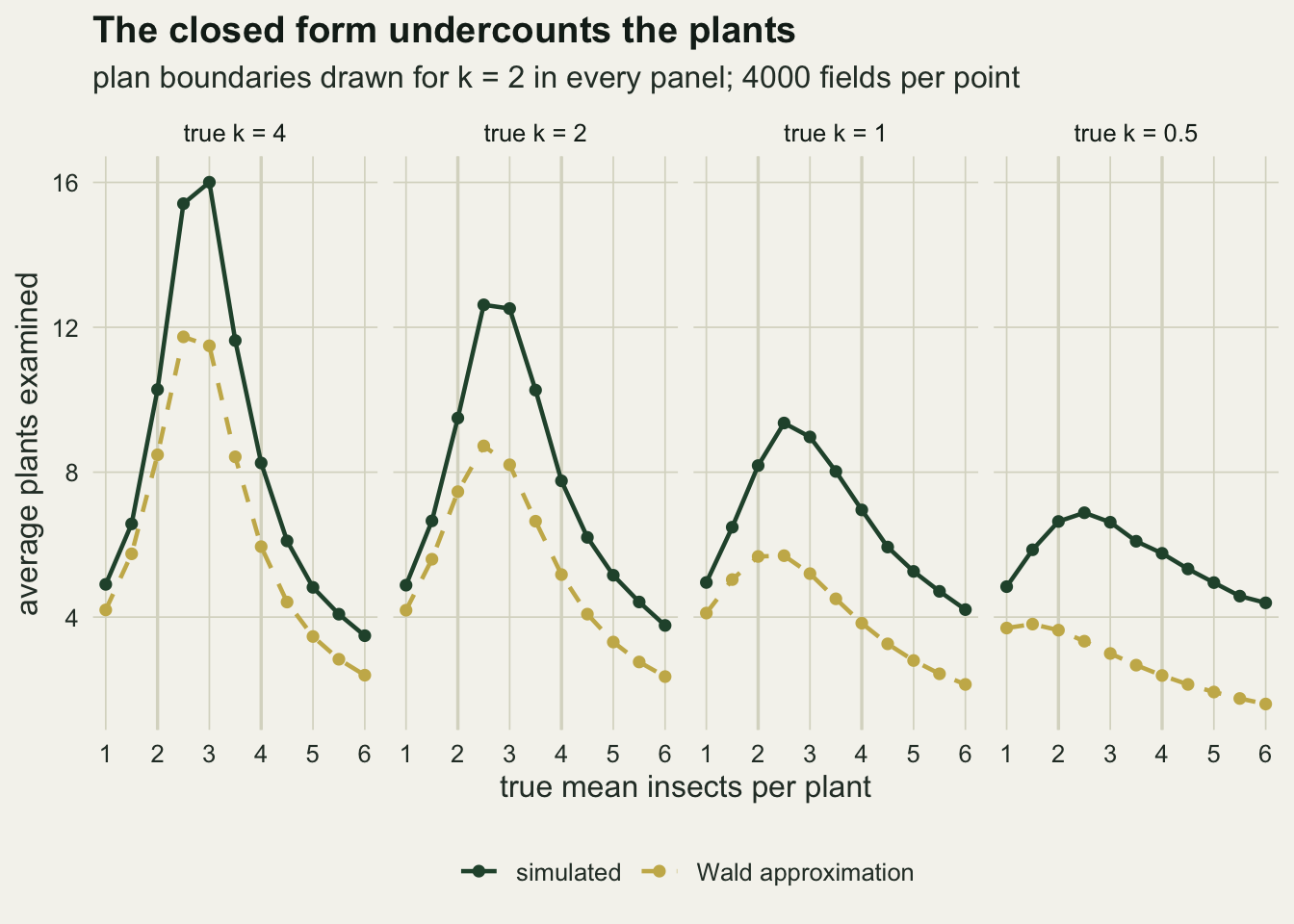
When the pest is more aggregated than assumed
Now keep the lines drawn for k = 2 and let the insects be clumped more strongly. This is the ordinary field situation: k is estimated once, from a pilot survey or a published table, and a given field on a given day can be far more patchy than that.
At a true k of 0.5 the plan treats a safe field in 0.175 of runs and misses an infested one in 0.337, while stopping after 6.64 and 5.76 plants on average. It stops sooner and is wrong more often. The mechanism follows from the shape of the counts: under strong aggregation many more plants are empty (0.45 of plants at a mean of 2 when k = 0.5, against 0.25 when k = 2), so a short run of empty plants carries the total across the lower line early, and the occasional heavily infested plant throws it across the upper line in one jump. The average drift per plant is the same at every k; what changes is how far single plants scatter the total. Both exits come before the plan has seen enough plants to know the mean.
Wald’s closed form, computed under the true k, gets the direction of all this right: it predicts 0.305 and 0.315 for the two error rates, both above nominal. It does not get the size right. It overstates the false treatment rate at the safe mean, slightly understates the missed infestations, and puts the average sample numbers at 3.64, 3.00 and 2.39 plants, short of the simulation by 45 to 59 per cent. Most of that gap comes through the error rates: fed the simulated rates instead of its own, the same formula gives 6.05 plants at the safe mean. The rest is overshoot, which is larger under aggregation because single plants move the total further past either line.
tay_0 <- pick("Taylor law", m0)
tay_1 <- pick("Taylor law", m1)
k_tay_0 <- k_taylor(m0)
k_tay_1 <- k_taylor(m1)
A single wrong k is the simplest version of the problem. Taylor’s power law says the variance scales as a m^b, which makes k move with the mean. With a = 2 and b = 1.5, fixed before the run, the implied k is 1.09 at the safe mean and 1.33 at the infested mean, so no single k is right and the assumed one is too high everywhere. The plan’s error rates are 0.094 and 0.132, between the k = 2 rates given above and the k = 1 rates of 0.107 and 0.185, which is where the implied k places them.
oc_df <- res
oc_df$scenario <- factor(oc_df$scenario, levels = c(paste("k =", k_grid), "Taylor law"))
oc_cols <- c("k = 4" = "#8fa89a", "k = 2" = te_forest, "k = 1" = te_gold,
             "k = 0.5" = te_rust, "Taylor law" = te_ink)

ggplot(oc_df, aes(m, p_treat, colour = scenario)) +
  annotate("rect", xmin = m0, xmax = m1, ymin = -Inf, ymax = Inf, fill = te_line, alpha = 0.35) +
  geom_line(aes(y = wald_treat), linetype = "dashed", linewidth = 0.5) +
  geom_line(linewidth = 0.9) +
  geom_point(size = 1.7) +
  geom_hline(yintercept = c(alpha_err, 1 - beta_err), linetype = "dotted", colour = te_body) +
  scale_colour_manual(values = oc_cols, name = "true aggregation") +
  scale_x_continuous(breaks = 1:6) +
  scale_y_continuous(limits = c(0, 1)) +
  labs(x = "true mean insects per plant", y = "probability of treating the field",
       title = "Clumping flattens the decision curve",
       subtitle = "solid: simulated; dashed: Wald; dotted: nominal 0.1 and 0.9 at means 2 and 4") +
  theme_datasheet() +
  theme(legend.position = "bottom")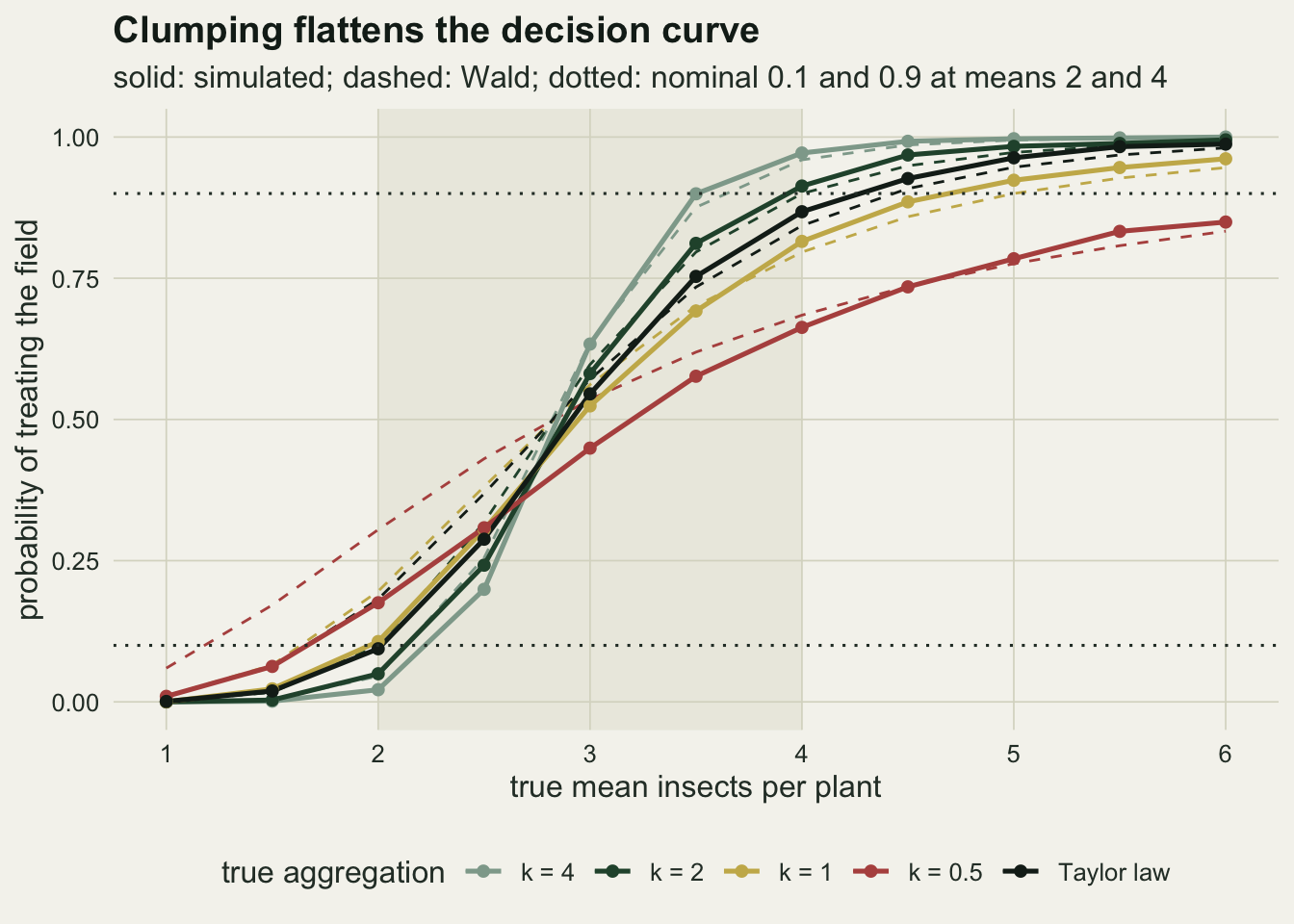
The fixed sample plan, given the same wrong k
The sequential plan is only worth its extra complexity if it saves plants against a plan that fixes n in advance. For that comparison to be fair, the fixed plan must be designed from the same assumed k and the same nominal errors, and then be exposed to the same true aggregation. The fixed plan counts n plants and treats when the total exceeds a cut. The sum of n independent negative binomial counts with common k is again negative binomial with size n k and mean n m, so its error rates come from pnbinom() exactly, with no simulation.
fixed_design <- function(k_plan, e0, e1) {
  for (n in 1:400) {
    cuts <- 0:(20 * n)
    ok <- which(pnbinom(cuts, size = n * k_plan, mu = n * m0, lower.tail = FALSE) <= e0 &
                pnbinom(cuts, size = n * k_plan, mu = n * m1) <= e1)
    if (length(ok) > 0) return(c(n = n, cut = cuts[ok[1]]))
  }
}
fixed_err <- function(plan, k_true) {
  c(err0 = pnbinom(plan[["cut"]], size = plan[["n"]] * k_true, mu = plan[["n"]] * m0,
                   lower.tail = FALSE),
    err1 = pnbinom(plan[["cut"]], size = plan[["n"]] * k_true, mu = plan[["n"]] * m1))
}

plan_nom  <- fixed_design(k_assumed, alpha_err, beta_err)
fix_k2    <- fixed_err(plan_nom, k_assumed)
fix_k05   <- fixed_err(plan_nom, 0.5)
plan_real <- fixed_design(k_assumed, r2_0$p_treat, 1 - r2_1$p_treat)

save_nom  <- 1 - c(r2_0$asn, r2_1$asn) / plan_nom[["n"]]
save_real <- 1 - c(r2_0$asn, r2_1$asn) / plan_real[["n"]]
save_mid_nom  <- 1 - r2_mid$asn / plan_nom[["n"]]
save_mid_real <- 1 - r2_mid$asn / plan_real[["n"]]
se_diff <- function(p) sqrt(p * (1 - p) / n_run)
z_safe <- (r05_0$p_treat - fix_k05[["err0"]]) / se_diff(r05_0$p_treat)
z_inf  <- ((1 - r05_1$p_treat) - fix_k05[["err1"]]) / se_diff(1 - r05_1$p_treat)
Designed at k = 2 for errors of one tenth, the fixed plan counts 13 plants and treats when the total exceeds 36. Its exact error rates at the right k are 0.081 and 0.098. The sequential plan’s average sample numbers of 9.49 and 7.76 are 27 and 40 per cent below that n, and near the threshold, at 12.52 plants, the saving shrinks to 4 per cent.
That comparison flatters the fixed plan, because the sequential plan also achieved lower errors than nominal. Holding the fixed plan to the error rates the sequential plan actually achieved at the right k, 0.050 and 0.087, needs 17 plants, and against that the saving is 44 and 54 per cent at the two design means and 26 per cent at the threshold. The rule of thumb that a sequential plan needs about half the samples of a fixed plan holds here only on that second, more generous comparison and only away from the threshold.
With the pest really at k = 0.5, the fixed plan of 13 plants errs in 0.169 of safe fields and 0.254 of infested ones. The sequential plan’s rates under the same misspecification were 0.175 and 0.337. On the safe side the two plans degrade to rates that differ by 1.0 Monte Carlo standard errors, which is no difference this simulation can resolve; on the infested side the sequential plan misses more fields, by 11 standard errors, because it is the one that stops early on a run of empty plants. The wrong k is not a special weakness of sequential sampling. It costs the sequential plan somewhat more, and it does so while also making the plan look cheaper.
cmp_df <- data.frame(
  plan   = rep(c("sequential", "fixed n"), each = 4),
  truth  = rep(rep(c("true k = 2", "true k = 0.5"), each = 2), 2),
  field  = rep(c("safe field, mean 2", "infested field, mean 4"), 4),
  wrong  = c(r2_0$p_treat, 1 - r2_1$p_treat, r05_0$p_treat, 1 - r05_1$p_treat,
             fix_k2[["err0"]], fix_k2[["err1"]], fix_k05[["err0"]], fix_k05[["err1"]]),
  plants = c(r2_0$asn, r2_1$asn, r05_0$asn, r05_1$asn, rep(plan_nom[["n"]], 4)))
cmp_df$truth <- factor(cmp_df$truth, levels = c("true k = 2", "true k = 0.5"))
cmp_df$field <- factor(cmp_df$field, levels = c("safe field, mean 2", "infested field, mean 4"))

ggplot(cmp_df, aes(plants, wrong, colour = plan, shape = truth)) +
  geom_hline(yintercept = alpha_err, linetype = "dotted", colour = te_body) +
  geom_line(aes(group = plan), colour = te_line, linewidth = 0.6) +
  geom_point(size = 3.2) +
  facet_wrap(~ field) +
  scale_colour_manual(values = c("sequential" = te_rust, "fixed n" = te_forest), name = NULL) +
  scale_shape_manual(values = c("true k = 2" = 16, "true k = 0.5" = 17), name = NULL) +
  scale_y_continuous(limits = c(0, NA)) +
  labs(x = "plants examined (average for the sequential plan)",
       y = "probability of the wrong decision",
       title = "Same wrong k, both plans pay",
       subtitle = "dotted: the nominal error of one tenth both plans were designed for") +
  theme_datasheet() +
  theme(legend.position = "bottom", legend.box = "vertical")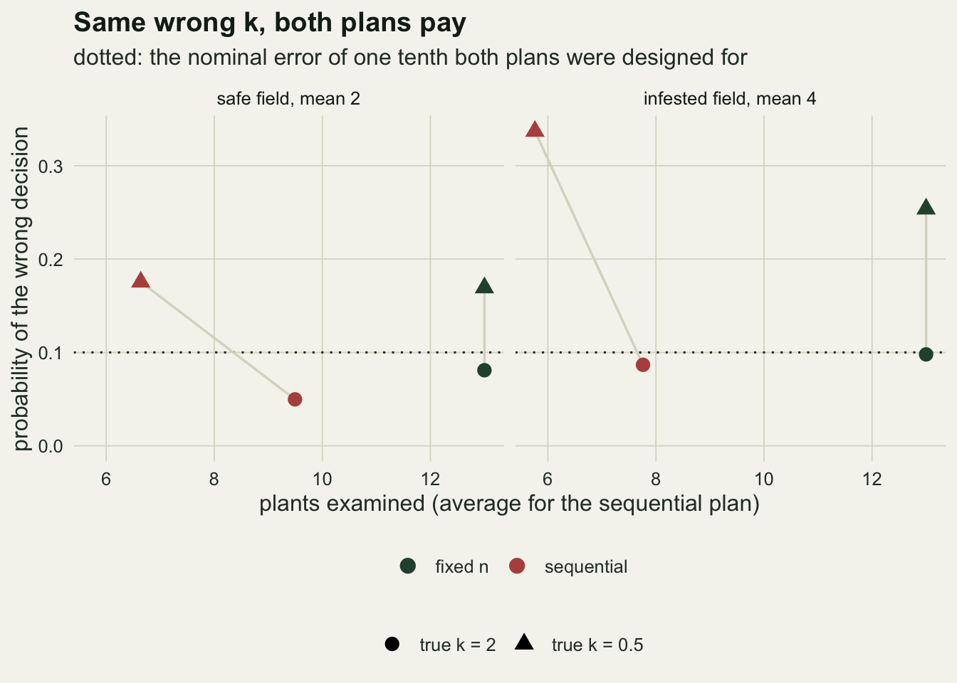
What the right k costs
set.seed(6630)
k05_0   <- run_plan(m0, 0.5, n_run, k_plan = 0.5)
k05_mid <- run_plan(3, 0.5, n_run, k_plan = 0.5)
k05_1   <- run_plan(m1, 0.5, n_run, k_plan = 0.5)
plan_k05 <- fixed_design(0.5, alpha_err, beta_err)
fix_k05_right <- fixed_err(plan_k05, 0.5)
ratio_seq <- c(k05_0[["asn"]] / r2_0$asn, k05_mid[["asn"]] / r2_mid$asn, k05_1[["asn"]] / r2_1$asn)
ratio_fix <- plan_k05[["n"]] / plan_nom[["n"]]
The repair is to draw the lines with the k the field actually has. With both the plan and the pest at k = 0.5, the error rates return to 0.056 and 0.099, and the average sample numbers become 24.2, 27.7 and 18.8 plants at true means 2, 3 and 4. Near the threshold the cap of 60 plants now binds in 0.112 of fields, so the forced decision at the cap carries part of the work. The fixed plan designed for the same k needs 34 plants for exact error rates of 0.099 and 0.095.
Against the plans for k = 2 at the right k, that is 2.2 to 2.5 times the plants for the sequential plan and 2.6 times for the fixed one. The honest price of aggregation is paid whichever plan is used, and the sequential plan drawn for k = 2 hides that price by stopping early and deciding badly.
What to report
State the k the boundaries were drawn with and where it came from: a pilot survey, a Taylor fit, or a published table for the pest and crop. The boundaries are uninterpretable without it, and two plans with the same threshold and error rates but different k are different plans.
Report the operating characteristic and average sample number from simulation, not from Wald’s formulas. The formulas are a check on the direction of an effect. For the sample number they fell short of the simulated value by 13 to 64 per cent across the whole grid of this measurement, and a plan’s cost in the field is its sample number.
Say what the plan does when it reaches its cap, and how often that happens at the threshold. A cap with a forced decision is a second rule inside the first one, and when the plan is drawn for a strongly aggregated pest it decides a noticeable share of the fields closest to the threshold.
Run the operating characteristic for at least one k below the assumed value. The spread between the k = 2 and k = 0.5 curves above is the sensitivity a user of the plan needs to see, and it is a five line addition to any simulation.
Honest limits
Only the Wald negative binomial plan was simulated. Current practice in integrated pest management also uses Iwao’s (1975) plan, which draws the boundaries from a regression of mean crowding on the mean instead of from a k, Green’s fixed precision stop lines, and presence and absence (binomial) plans that count infested plants rather than insects, which are faster in the field and trade information for speed. Binns and Nyrop (1992) review all of them. None was tested here, and nothing above says how they behave under the same misspecification; the binomial plans in particular depend on the relationship between the mean and the proportion of infested plants, which aggregation also shifts.
Plants were independent draws from one negative binomial with one mean. A real walk crosses edges, headlands and hot spots, and a mean that changes along the path violates the identically distributed assumption of the likelihood ratio in a way that a wrong k does not describe. Sampling patterns (a W or a zigzag across the field) exist to limit this, and they were not simulated.
The Taylor law scenario used one pair of constants chosen before the run, and the scenarios with a fixed wrong k covered one assumed value. The size of the error inflation depends on both. The claim that holds across the runs here is directional: more aggregation than assumed made the plan stop sooner at the design means and the threshold, and err more at both design means (at a mean of 1 the sample numbers are indistinguishable).
The fixed plan was evaluated exactly, the sequential plan by simulation with 4000 fields per cell, so the sequential rates carry Monte Carlo standard errors of up to 0.0079 and the fixed ones carry none. That is why the safe-field comparison with the fixed plan was read as no difference and the infested-field one was not.
The decision was treated as two errors with fixed rates. A manager who sets the threshold from the cost of spraying and the cost of yield loss is solving the problem in choosing a decision threshold from costs, and the error rates of a sampling plan are then an input to that calculation rather than a target in themselves.
References
Wald A 1945 Annals of Mathematical Statistics 16(2):117-186 (10.1214/aoms/1177731118)
Iwao S 1975 Researches on Population Ecology 16(2):281-288 (10.1007/BF02511067)
Binns MR, Nyrop JP 1992 Annual Review of Entomology 37:427-453 (10.1146/annurev.en.37.010192.002235)
Taylor LR 1961 Nature 189(4766):732-735 (10.1038/189732a0)